1 Introduction

“...the campaign to discredit the press works by generating noise and confusion...”
(Jay Rosen, “Why Trump Is Winning and the Press Is Losing,” New York Review of Books online, April 15, 2018)

Consider a politician who seeks to discredit information, to prevent people from becoming well-informed about an inconvenient truth. Can the politician achieve this goal even when people are rational and perfectly understand the politician’s incentives? Should we be optimistic that new social media technologies will make it more difficult for the politician to discredit inconvenient reporting? Or will these new technologies make it easier for the politician to create confusion, frustrating people in their desire to be well-informed?¹

We develop a simple model to answer these questions. There is a collection of citizens each of whom seeks to form an accurate assessment of an underlying state using the sources of information available to them. An informed politician seeks to discredit the citizens’ information, at a cost. The citizens are rational and internalize the politician’s incentives.

We interpret the social media revolution as a shock that simultaneously: (i) increases the underlying, intrinsic precision of the information available to the citizens, and (ii) decreases the costs the politician incurs in manipulating information. We argue that these new technologies have led to new sources of information, both in the form of new media outlets and in the form of blogging and amateur journalism, thereby increasing the intrinsic precision of the information available to citizens, but that these new sources of information are not all subject to the same standards of accountability as traditional media and moreover are consumed in a feed that blurs distinctions between outlets and that makes it easier for all kinds of news, real and fake, to “go viral,” thereby reducing the costs of manipulation.

We find that the social media revolution can generate a “regime change” in the amount of manipulation: The net effect of the shock depends on whether the costs of manipulation can be kept above a critical threshold. If the intrinsic precision of information is high and the costs of manipulation fall below this critical threshold, the economy will enter a high manipulation regime. In this high manipulation regime, the politician’s manipulation prevents improvements in the intrinsic precision from passing through to citizens, making them worse off and the politician better off. But if the costs of manipulation can be kept above this critical threshold the economy will stay in a low manipulation regime. In this low manipulation regime, the politician fails to prevent improvements in the intrinsic precision from passing through to the citizens, making the citizens better off and the politician worse off.

Section 2 outlines the model. There is a politician who knows the underlying state of the world. There is a continuum of citizens who share a common prior and receive idiosyncratic signals about the state. Each citizen wants to take an action that is appropriate for the state and the politician seeks to prevent them from doing so. Thus in contrast to standard political economy models, the citizens’ and politician’s interests are not even partially aligned. The politician has a technology that allows them to manipulate information by choosing the citizens’ signal mean at a cost that is increasing in the distance between the true state and the signal mean. The citizens are rational and internalize the politician’s incentives. To keep the model tractable, we assume quadratic preferences and normal priors and signal distributions. We study equilibria that are linear in the sense that the citizens’ strategies are linear functions of their signals.

Section 3 solves the model and shows that there is a unique (linear) equilibrium. In equilibrium, the citizens’ signals are unbiased but are made endogenously noisier by the politician’s manipulation. The equilibrium amount of manipulation can be very sensitive to parameters. If the costs of manipulation are high, increasing the intrinsic precision decreases the amount of manipulation and the citizens become more responsive to their signals than they would be if the politician could not manipulate at all. But if the costs of manipulation are low, increasing the intrinsic precision increases the amount of manipulation and citizens are less responsive to their signals than they would be in the absence of manipulation. Moreover we show that if the intrinsic precision of information is high there is a critical threshold for the costs of manipulation. At this threshold, a small change in the costs of manipulation causes a discontinuous jump in the amount of manipulation, giving rise to the possibility of abrupt transitions between low manipulation and high manipulation regimes.

Section 4 contains our results on the welfare effects of a social media revolution, interpreted as a simultaneous increase in the intrinsic signal precision and decrease in the costs of manipulation. The net effect of the social media revolution depends crucially on the size of the reduction in the costs of manipulation. If the costs fall enough, the economy tips into the high manipulation regime, where no change in the intrinsic signal precision can compensate the citizens’ for the welfare loss brought by the fall in the costs of manipulation. Indeed in the limit where the costs of manipulation become negligible, the politician’s manipulation renders the citizens’ signals completely uninformative even if the underlying, intrinsic precision of their signals is arbitrarily high. But if the costs of manipulation do not fall too much, the citizens eventually benefit from the increase in the intrinsic signal precision. In this sense, even small changes on the part of social media platforms that make it harder for misinformation to propagate may have large welfare effects.

Section 5 discusses two extensions of our benchmark model. First we outline a version of our model where citizens do not simply consume signals but rather consume media reports produced by journalists that have their own preferences that need not be perfectly aligned with the citizens. Each journalist cares both about reporting the truth and about how their report fits with other reports (their actions may be either strategic substitutes or complements). In this version of the model the politician is directly concerned with manipulating the journalists’ information with the citizens affected as a byproduct. This setting gives rise to some new possibilities. For one, the politician’s manipulation can backfire if there are sufficiently strong strategic interactions amongst the journalists, i.e., there are scenarios where the politician would value being able to commit to not manipulate information. For another, we find that the citizens can benefit from the politician’s manipulation if the journalists’ actions are strong strategic substitutes and the intrinsic precision of their signals is sufficiently low. That said, regardless of the strength of strategic interactions among the journalists, the politician gains the most and the citizens lose the most when the costs of manipulation are low and the intrinsic precision of the signals is high, as in our benchmark model.

Second, we outline a version of the model where citizens have heterogeneous priors and where the politician can directly manipulate both the signal mean and the signal variance. We use this setting to analyze an alternative notion of better information, namely a reduction in prior dispersion. We again find that the politician’s manipulation can prevent this better information from passing through to the citizens.

Interpretation. Our model is intended to capture features of political messaging that used to be known by terms like “muddying the waters” but more recently has become known as the “politics of confusion”. Pomerantsev (2019) discusses such political messaging at length and explains how it has been used by authoritarian regimes around the world to consolidate power and to sow doubts about democratic institutions (see also Bennett and Livingston (2018) and Sunstein (2018) amongst others). In democracies, this form of political messaging has come under considerable scrutiny since the 2016 UK Brexit referendum and the 2016 US presidential election, as voters found themselves on the receiving end of a relentless deluge of spin and “alternative facts” especially as propagated via social media. More systematically, Bradshaw and Howard (2019) and Nyst and Monaco (2018) document evidence of organized social media manipulation by governments and political parties in 70 countries, covering both democracies and autocracies. According to these reports, the goal of the organized social media manipulation is to confuse the very notion of truth, sow seeds of distrust in the media, discredit criticism and oppositional voices, and drown out political dissent.

But there is also a competing, more benevolent, view of the role played by social media. After all it was not so long ago that the conventional wisdom was the other way round, arguing that social media is a force for transparency and democratic accountability (see e.g., (Shafer 2010) on WikiLeaks) and helping to bring about important social and political reforms (see e.g., (Codrea-Rado 2017) and Rickford (2015) on #BlackLivesMatter and #MeToo).

Our model interprets these competing views in the following way. Absent manipulation, new social media technologies would allow people to make more informed decisions, making them better off. But in the presence of manipulation, these new technologies also reduce the politician’s costs of manipulation, thereby creating a tension. Our results then provide a characterization of the net effects of this tension, allowing us to say when people will and will not be better off overall.

Strategic communication with costly talk. Our model is a sender/receiver game with many imperfectly informed receivers.² As in Crawford and Sobel (1982), the preferences of the sender and receivers are not aligned and the sender is informed. But as in Kartik (2009) we have costly talk, not cheap talk. By contrast with standard cheap talk models, our model with costly talk features a unique equilibrium. In the limit as the sender’s distortion becomes almost costless, the unique equilibrium features a kind of babbling where the receivers ignore their signals. Our model with costly talk is related to Kartik et al. (2007) and Little (2017) but our receivers are not “credulous” or subject to confirmation bias.

Bayesian persuasion. In equilibrium, our receivers have unbiased posterior expectations. Despite this, the sender still finds it optimal to send costly distorted messages. This is because of the effects of their messages on other features of the receivers’ beliefs, as in the Bayesian persuasion literature following Kamenica and Gentzkow (2011, 2014). In particular, the sender can be made better off by the increase in the receivers’ posterior variance resulting from the sender’s messages. A crucial distinction however is that in Kamenica and Gentzkow (2011), the sender can commit to an information structure and this commitment makes the model essentially nonstrategic in that their receiver only needs to solve a single-agent decision problem. Other approaches to information design, such as Bergemann and Morris (2016) also allow the sender to commit. By contrast, our sender cannot commit and chooses their message after becoming informed about the underlying state, as in Crawford and Sobel (1982).

Applications to political communication that follow the Bayesian persuasion approach in assuming the sender can commit include Hollyer et al. (2011), Gehlbach and Sonin (2014), Gehlbach and Simpser (2015) and Rozenas (2016). In terms of the sender not being able to commit, our model is more similar to Little (2012, 2015) and Shadmehr and Bernhardt (2015) but we differ from Little (2012) in that our sender is informed, and from Shadmehr and Bernhardt (2015) in that the sender uses a distinct information manipulation technology. Other related work includes Egorov et al. (2009), Edmond (2013), Lorentzen (2014), Huang (2015), Guriev and Treisman (2015), and Chen and Xu (2017). For overviews of this literature, see Svolik (2012) and Gehlbach et al. (2016).

Media bias, fake news, and alternative facts. The media bias literature often assumes that receivers prefer distorted information³ — e.g., Mullainathan and Shleifer (2005), Baron (2006), Besley and Prat (2006), Gentzkow and Shapiro (2006), Bernhardt et al. (2008) and Martin and Yurukoglu (2017). Allcott and Gentzkow (2017) and Gentzkow et al. (2015) have used this kind of setup to explain how there can be a viable market for “fake news” that coincides with more informative, traditional media. To be clear, we view such behavioral biases as very important. Our point is that such biases are not necessary for manipulation to be effective. In our model, the sender can still gain from sending costly distorted messages because of the endogenous noise that results from such messages.

Or to put things a bit differently, in our model no one is misled by the politician’s “alternative facts” and yet the politician can benefit greatly from the ensuing babble and tumult.

2 Model

There is a unit mass of ex ante identical citizens, indexed by \(i\in[0,1]\), and a single informed politician attempting to influence their beliefs.

Citizens. Each individual citizen wants to take an action \(a_i\in\mathbb{R}\) that is appropriate for the underlying state \(\theta\in\mathbb{R}\) (about which they are imperfectly informed). In particular, each citizen chooses \(a_i\) to minimize the expected value of the quadratic loss \[\tag{1} (a_i-\theta)^2\] so that each citizen sets their action \(a_i\) equal to their expectation of \(\theta\).

In forming expectations of \(\theta\), the citizens begin with the common prior that \(\theta\) is distributed normally with mean \(z\) and precision \(\alpha_z>0\) (i.e., variance \(1/\alpha_z\)). Each individual citizen then draws an idiosyncratic signal \[x_i=y+\varepsilon_i \tag{2}\] where the mean \(y\) is chosen by the politician, as discussed below, and where the idiosyncratic noise \(\varepsilon_i\) is IID normal across citizens, independent of \(\theta\), with mean zero and precision \(\alpha_x>0\) (i.e., variance \(1/\alpha_x\)). Based on this information, each citizen sets their action to \[\tag{3} a_i = \mathbb{E}[\theta\,|\,x_i ]\]

To summarize, the citizens have one source of information, the prior, that is free of the politician’s influence and another source of information, the signal \(x_i\), that is not. While the informativeness of the prior is fixed, the informativeness of the signal needs to be determined endogenously in equilibrium in light of the politician’s incentives.

Politician. The politician knows the value of \(\theta\) and seeks to prevent the citizens from forming expectations that are accurate for the underlying state \(\theta\). In particular, the politician obtains a gross benefit \[\int_0^1\,(a_i-\theta)^{2}\,di \tag{4}\]that is increasing in the dispersion of the actions \(a_i = \mathbb{E}[\theta\,|\,x_i ]\) around \(\theta\).⁴ The politician is endowed with the ability to choose the mean \(y\) of the citizens’ idiosyncratic signals. In particular, knowing \(\theta\), the politician may take a costly action \(s\in \mathbb{R}\) to make the signal mean \(y=\theta+s\), i.e., the term \(s=y-\theta\) can be interpreted as the slant or spin that the politician is attempting to introduce. This manipulation incurs a quadratic cost \(c(y-\theta)^{2}\), similar to Holmström (1999) and Little (2012, 2015), so that the net payoff to the politician is \[V=\int_0^1\,(a_i-\theta)^{2}\,di-c(y-\theta )^{2},\qquad c>0 \tag{5}\]where the parameter \(c>0\) measures how costly it is for the politician to choose values of \(y\) far from \(\theta\). The special case \(c\rightarrow 0\) corresponds to a version of cheap talk (i.e., the politician can choose \(y\) arbitrarily far from \(\theta\) without cost). The special case \(c\rightarrow \infty\) corresponds to a setting without manipulation (i.e., where the politician will always choose \(y=\theta\)).

Equilibrium. A symmetric perfect Bayesian equilibrium of this model consists of individual citizen actions \(a(x_i)\) and beliefs and the politician’s manipulation \(y(\theta)\) such that: (i) each citizen rationally takes the manipulation \(y(\theta)\) into account when forming their beliefs, (ii) each citizen’s action \(a(x_i)\) minimizes their expected loss, and (iii) the politician’s \(y(\theta)\) maximizes the politician’s payoff given the individual actions.

Before characterizing equilibrium outcomes in the general model with information manipulation, we first review equilibrium outcomes when there is no manipulation.

Equilibrium with no manipulation. Suppose the politician cannot manipulate information — i.e., let \(c\rightarrow \infty\) so that the politician chooses \(y=\theta\). This puts us in a standard linear-normal setting where each citizen’s posterior expectation of \(\theta\) is a precision-weighted average of their signal \(x_i\) and prior \(z\). In particular, the optimal actions are given by \[a(x_i)=\mathbb{E}[\, \theta \,|\,x_i\,]=\frac{\alpha_x}{\alpha _x+\alpha_z} x_i+\frac{\alpha_z}{\alpha_x+\alpha_z}z . \tag{6}\] For future reference, let \[k_{nm}^* := \frac{\alpha}{\alpha+1},\qquad \alpha:=\frac{\alpha_x}{\alpha_z}>0 \tag{7}\] denote the response of each citizen to their signal when there is no manipulation. This response coefficient is determined by the relative precision \(\alpha\) of the signal to the prior.

3 Equilibrium with Information Manipulation

Now suppose the politician can manipulate information. In this setting there is a genuine equilibrium fixed-point problem because we need to ensure that the citizens’ actions and beliefs and the politician’s information manipulation are mutually consistent.

Preliminaries. We restrict attention to equilibria in which the citizens use symmetric linear strategies. We write these as \[a(x_i)=k x_i+(1-k)z \tag{8}\] The fact that the citizens’ strategies are linear is a genuine restriction. But, as we show in our Supplementary Online Appendix, the fact that the coefficients sum to one is a result and it streamlines the exposition to make use of this result from the start.

3.1 Politician’s Problem

Given that the citizens use linear strategies \(a(x_i)=kx_i+(1-k)z\), the politician’s problem is to choose \(y\in \mathbb{R}\) to maximize \begin{align} V(y) &= \int_0^1 \big( \, k(y+\varepsilon_i) + (1-k)z -\theta \, \big)^2 \, di - c(y-\theta)^2 \notag \\ & \notag \\ & = (ky + (1-k)z - \theta)^2 + \frac{1}{\alpha_x} k^2 - c(y-\theta)^2 \tag{9} \end{align} Taking the citizens’ response coefficient \(k\) as given, this is a simple quadratic optimization problem. The solution is \[\tag{10} y(\theta) = \frac{c-k}{c-k^2} \theta + \frac{k-k^2}{c-k^2} z\] where the second-order condition requires \[\tag{11} c-k^2 \geq 0\] Given that the citizens use linear strategies, it is optimal for the politician to also use a linear strategy. The coefficients in the politician’s strategy sum to one, so we can write \[\tag{12} y(\theta) = (1-\delta)\theta + \delta z\] where \(\delta\) depends on the citizens’ response coefficient \(k\) via \[\tag{13} \delta(k) := \frac{k-k^2}{c-k^2},\qquad c-k^2\geq0\] To interpret the politician’s strategy, observe that if, for whatever reason, the politician chooses \(\delta(k)=0\), then the politician is choosing a signal mean \(y\) that coincides with the true \(\theta\) — i.e., the politician chooses not to manipulate information and the citizens’ signals \(x_i\) are as informative as possible about the true \(\theta\) (limited only by the intrinsic precision, \(\alpha_x\)). Alternatively, if the politician chooses \(\delta(k)=1\), then the politician is choosing a signal mean \(y\) that coincides with the citizens’ prior \(z\) — i.e., the citizens’ signals \(x_i\) provides no additional information about \(\theta\).

In short, the politician’s manipulation coefficient \(\delta(k)\) summarizes the politician’s best response to the citizens’ coefficient \(k\). To construct an equilibrium, we need to pair this with the citizens’ best response to the politician’s manipulation.

3.2 Citizens’ Problem

To construct the citizens’ best response, first observe that the optimal action \(a(x_i)\) for an individual with signal \(x_i\) is given by \(a(x_i)=\mathbb{E}[\, \theta \,|\,x_i]\). Our task now is to characterize these expectations. If the politician’s manipulation strategy is (12), then each individual citizen has two pieces of information: (i) the common prior \(z=\theta+\varepsilon_z\), where \(\varepsilon_z\) is normal with mean zero and precision \(\alpha_z\), and (ii) the idiosyncratic signal \begin{align} x_i=y(\theta)+\varepsilon_i& =(1-\delta)\theta +\delta z+\varepsilon_i \notag \\ & \notag \\ & =\theta +\delta \varepsilon_z+\varepsilon_i \tag{14}\end{align}where the \(\varepsilon_i\) are IID normal with mean zero and precision \(\alpha_x\). The key point is that the politician’s manipulation \(\delta\) makes the signal \(x_i\) less correlated with the true \(\theta\) and more correlated with the prior \(z\). To extract the dependence on the prior, we construct a synthetic signal \[\hat{x}_i:=\frac{1}{1-\delta }\left(x_i-\delta z\right) =\theta +\frac{1}{1-\delta }\varepsilon_i \tag{15}\] The synthetic signal \(\hat{x}_i\) is independent of the prior and normally distributed around the true \(\theta\) with precision \((1-\delta)^{2}\alpha_x\). If \(\delta=0\), such that \(y(\theta)=\theta\), there is no manipulation from the politician and hence the synthetic signal \(\hat{x}_i\) has precision \(\alpha_x\), i.e., equal to the intrinsic precision of the actual signal \(x_i\). If \(\delta =1\), such that \(y(\theta)=z\), the signal \(x_{i}\) is uninformative about \(\theta\) and the synthetic signal has precision zero.

Conditional on the synthetic signal \(\hat{x}_i\), an individual citizen has posterior expectation \[\tag{16} \mathbb{E}[\, \theta \,|\,\hat{x}_i]=\frac{(1-\delta)^{2}\alpha_x}{(1-\delta)^{2}\alpha_x+\alpha_z}\hat{x}_i+\frac{\alpha_z}{(1-\delta)^{2}\alpha_x+\alpha_z}z\] So in terms of the actual signal \(x_i\) they have \[\tag{17} \mathbb{E}[\, \theta \,|\,x_i]=\frac{(1-\delta)\alpha_x}{(1-\delta)^{2}\alpha_x+\alpha_z}x_i+\left(1-\frac{(1-\delta)\alpha_x}{ (1-\delta)^{2}\alpha_x+\alpha_z}\right) z.\] Hence indeed the citizens have a strategy of the form \[ a(x_i) = kx_i + (1-k)z\] where the response coefficient \(k\) is given by \[k(\delta):=\frac{(1-\delta )\alpha}{(1-\delta)^{2}\alpha +1} \tag{18}\]and where again \(\alpha :=\alpha_x/\alpha_z\) is the intrinsic precision of the signal relative to the prior.

To summarize, citizens have strategies of the form \(a(x_i)=k x_i+(1-k)z\) where the response coefficient \(k\) is a function of the politician’s manipulation \(\delta\) and the politician has a strategy of the form \(y(\theta)=(1-\delta)\theta +\delta z\) where the manipulation coefficient \(\delta\) is a function of the citizens’ \(k\). Think of these as two curves, \(k(\delta)\) for the citizens and \(\delta(k)\) for the politician. Finding equilibria reduces to finding points where these two curves intersect.

Before characterizing equilibria in this way, we briefly discuss the model.

3.3 Discussion

Politician’s preferences. In our model, the politician benefits at the expense of the citizens, specifically, when the citizens take actions that diverge from the true \(\theta\). This makes our setup distinct from traditional political economy models where citizens’ and politicians’ interests are at least partially aligned. We introduce this non-standard setup to capture the emerging phenomenon of political messaging known as the politics of confusion. To see how the politics of confusion fits in with more traditional political economy models, consider the following three scenarios.

First, consider an opposition leader who sincerely believes that the citizens will be better off if she rather than the incumbent wins an election. This kind of “ends justify the means” thinking rationalizes the use of the politics of confusion to help win the election. In other words, although there may be an interim conflict of interest, there is, at least in the opposition leader’s mind, no ultimate conflict of interest. Second, consider a politician who is highly effective at economic policy, delivering reforms that improve the livelihoods of millions of people, but who is at the same time personally corrupt and seeks to prevent citizens from becoming informed about the extent of the corruption. In other words, politicians and citizens have multidimensional interests and while they may be aligned along many dimensions they may be in conflict along others. Finally, consider a foreign political leader who seeks to sow confusion and doubt in the minds of the domestic political audience of a rival country. Here the conflict of interest is simple and genuine.⁵

To illustrate more generally what we mean by the politics of confusion, consider the following three examples:

Example 1. “In Britain there is no consistent political narrative, no clear party lines and for many people no way to see what is truth, lie, conspiracy or paranoia. There are just squabbling factions and confusion. While in Russia this situation was (at least partially) orchestrated, in Britain this has occurred through groups and individuals manoeuvring for power and their own interests but the results are the same: confusion and the potential for manipulation.” (Till 2016)

Example 2. “But I soon found myself reflexively questioning every headline. It wasn’t that I believed Trump and his boosters were telling the truth. It was that, in this state of heightened suspicion, truth itself — about Ukraine, impeachment, or anything else — felt more and more difficult to locate. With each swipe, the notion of observable reality drifted further out of reach. What I was seeing was a strategy that has been deployed by illiberal political leaders around the world. Rather than shutting down dissenting voices, these leaders have learned to harness the democratizing power of social media for their own purposes – jamming the signals, sowing confusion. They no longer need to silence the dissident shouting in the streets; they can use a megaphone to drown him out. Scholars have a name for this: censorship through noise.” (Coppins 2020).

Example 3. “The strategic objective remains the same — to weaken and destabilize the West — but today’s Russia is no longer seeking to be an ideological challenger to the West in the way that the Soviet Union had. The Kremlin is not out to prove that its model is superior to liberal democracy. Now, it is enough to sow doubt in Western institutions and confuse the very notion of truth with a barrage of alternative narratives mixing fact, distortions, and outright fabrications.” (Polyakova and Fried 2018).

Finally, note that in our model the politician has no “directional bias” — they are not trying to tilt the citizens’ beliefs in a particular direction. If the politician tried to inject a known directional bias (to the left or right, say) into their messaging, that would be easily extracted by the citizens in forming their beliefs about \(\theta\). This would end up increasing the politician’s marginal costs but otherwise leave the analysis unchanged. We think of our model as pertaining to the residual uncertainty after known biases have been extracted.

Politician’s manipulation strategy. The politician’s manipulation strategy turns a signal centered on the truth into a signal centered on a mixture of the truth and the citizens’ prior prejudice. This represents the systematic provision of an alternative information environment that undermines the credibility of the intrinsic information available to the citizens. Examples of such information manipulation include attacks on the news media in public speeches and tweets (Downie, Jr. 2020), contradictory allegations of fake news, half truths, and disputed facts through Facebook and Twitter (Goldhill 2019), pushing out many versions of “alternative narratives” through state media, officials, and social media accounts (Polyakova and Fried 2018), and orchestrating a multitude of contradictory political characters and stories (Ratcliffe 2016).

In our model, this manipulation strategy will not, in equilibrium, lead to any bias in the citizens’ beliefs about \(\theta\). Instead, the politician’s manipulation makes the signals \(x_i\) endogenously noisier than they otherwise would be, preventing the benefits of intrinsically precise information from passing through to the citizens. In equilibrium, the citizens receive unbiased information yet at the same time they will feel frustrated, getting information that is less informative than it could be, with the politician able to benefit from the reduced credibility of the media.

Costs of manipulation. We interpret the costs of manipulation as the real resources spent on providing the citizens with the alternative information environment, an environment that combines a mixture of true facts and “alternative facts" or misdirection. In the pre-social media era, the costs of manipulation would include the resource costs of running a large state-controlled mass media. But the rise of social media has brought new tools for manipulating information that are implemented through “cyber troops" employed by the states or strategic communications firms. According to Bradshaw and Howard (2019), the size and permanency of these “cyber troops” varies considerably across countries, from temporary teams with a handful of personnel who manage a few hundred fake social media accounts to vast permanent teams organized in local and regional offices. These contracts with strategic communication firms can range from smaller spends with boutique national or regional firms, to multi-million-dollar contracts with global companies like Cambridge Analytica.

3.4 Equilibrium Determination

Recall that citizens have strategies of the form \(a(x_i)=k x_i+(1-k)z\) where the response coefficient is a function \(k(\delta)\) of the politician’s manipulation and the politician has a strategy of the form \(y(\theta)=(1-\delta)\theta +\delta z\) where the manipulation coefficient is a function \(\delta(k)\) of the citizens’ response. Finding equilibria reduces to finding points where the \(k(\delta)\) and \(\delta(k)\) curves intersect. Let \(k^*\) and \(\delta^*\) denote such equilibrium points.

Now define \[\mathcal{K}(c):=\{ \,k\,:\,0\leq k\leq \min [c,1]\, \},\qquad c>0 \tag{19}\] This is the set of \(k\) such that \(\delta(k)\in[0,1]\). The upper bound \(k\leq \min[c,1]\) comes from the fact that if \(c\leq1\) then \(\delta(k)\leq 1\) if and only if \(k\leq c\). We can now state our first main result:

Figure 1 illustrates the result, with \(k\) on the horizontal axis and \(\delta\) on the vertical axis. In general, both these curves are non-monotone but they intersect once, pinning down a unique pair \(k^*,\delta^*\) from which we can then determine the politician’s equilibrium strategy \(y(\theta)=(1-\delta^*)\theta +\delta^* z\) and the citizens’ equilibrium strategy \(a(x_i)=k^* x_i+(1-k^*) z\).

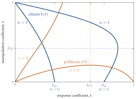
There is a unique equilibrium, that is, a unique pair \(k^*,\delta^*\) simultaneously satisfying the citizens’ best response \(k(\delta)\) and the politician’s best response \(\delta(k)\). For \(\alpha>1\) there is a critical point \(\hat{\delta}(\alpha)\) such that the citizens’ \(k(\delta)\) is increasing in \(\delta\) for \(\delta<\hat{\delta}(\alpha)\). For \(c>1\) there is a critical point \(\hat{k}(c)\) such that the politician’s \(\delta(k)\) is decreasing in \(k\) for \(k>\hat{k}(c)\). Note that if \(c<1\) then \(k^*\leq c\) and hence \(k^*\) cannot be high if \(c\) is low.

Open this figure on its own page

When is the citizens’ best response non-monotone?

Lemma 1 says that if \(\alpha\) is relatively high and the amount of manipulation \(\delta\) is relatively low, then the citizens will in fact be more responsive to their signals than they would be in the absence of manipulation. To understand why this can happen, we need to decompose the effect of \(\delta\) into two parts: (i) the effect of \(\delta\) on the precision of the synthetic signal \(\hat{x}_i\) in (15), and (ii) the effect of \(\delta\) on the correlation between the citizens’ actual signal \(x_i\) and their prior \(z\). We will refer to the former as the “precision ” effect and to the latter as the “correlation ” effect. From (15), the synthetic signal precision is \((1-\delta)^2 \alpha_x\) and hence is unambiguously decreasing in \(\delta\). This reduction in precision acts to decrease the citizens’ \(k\). But an increase in \(\delta\) also increases the correlation between \(x_i\) and \(z\). Since \(z\) also contains information about the fundamental \(\theta\), this increase in correlation acts to increase the citizens’ response to their signals \(x_i\). For \(\alpha \leq 1\), the precision effect unambiguously dominates so that \(k(\delta)\) is strictly decreasing from \(k(0)=k^*_{nm}\) to \(k(1)=0\). For \(\alpha>1\), the correlation effect dominates for low levels of \(\delta\) while the precision effect dominates for high levels of \(\delta\) so that \(k(\delta)\) increases from \(k(0)=k^*_{nm}\) to its maximum then decreases to \(k(1)=0\).

That said, the bottom line is that for high enough manipulation, it will indeed be the case that the citizens are less responsive to their signals, \(k(\delta)<k_{nm}^*\). This hurdle is easy to clear when \(\alpha\) is relatively low, but hard to clear when \(\alpha\) is relatively high.

When is the politician’s best response non-monotone?

Lemma 2 says that if the costs of manipulation are relatively low, then whenever the citizens respond more to their signals, the politician will choose a higher level of manipulation.⁶ But if instead the costs of manipulation are relatively high, then for high enough \(k\) the politician responds by choosing a lower level of manipulation \(\delta(k)\).⁷

To understand why higher values of the citizens’ response coefficient \(k\) can lead the politician to choose less manipulation, we first write the politician’s gross payoff as \[ \int_0^1 \, (a_i-\theta)^2 \,di = (A-\theta)^2 + \int_0^1 \, (a_i-A)^2 \,di\] In short, the politician can be made better off through either increasing the distance between \(A\) and \(\theta\) or through increasing the dispersion of \(a_i\) around \(A\). Now observe that if the politician uses the strategy \(y=(1-\delta)\theta+ \delta z\) then \(A-\theta=(k\delta+1-k)(z-\theta)\), proportional to the error in the common prior \(z-\theta\). Similarly if the citizens use the strategy \(a_i=kx_i+(1-k)z\) then \(a_i-A = k(x_i - y) = k\varepsilon_i\), proportional to the idiosyncratic noise \(\varepsilon_i\). The politician’s choice of \(\delta\) enters the gross payoff only through the term \((A-\theta)^2\).

Subtracting off the cost \(c(y-\theta)^2\) and collecting terms gives the politician’s objective \[\tag{22} V = \big(B(\delta,k) - C(\delta) \big) (z-\theta)^2 + \frac{1}{\alpha_x}k^2\] where \(B(\delta,k):=(k\delta+1-k)^2\) denotes the benefit the politician obtains from increasing the distance between \(A\) and \(\theta\), and \(C(\delta):=c \delta^2\) denotes the associated costs. We can now view the politician’s problem as being equivalent to choosing \(\delta\in [0,1]\) to maximize (22) taking \(k\in[0,1]\) as given. Notice that \(k\) affects the optimal \(\delta\) only through the marginal benefit \[\tag{23} \frac{\partial B}{\partial \delta } = 2(k \delta + 1-k)k\] Now recall that \(A-\theta=(k\delta+1-k)(z-\theta)\) so the term \((k\delta+1-k)\) is simply the coefficient on the error in the common prior. There are then two effects of an increase in \(k\) on the the marginal benefit: (i) an increase in \(k\) makes the coefficient \((k\delta+1-k)\) more sensitive to \(\delta\), which increases the marginal benefit of manipulation, but also (ii) an increase in \(k\) decreases the magnitude of \((k\delta+1-k)\), which decreases the marginal benefit of manipulation. When the first effect dominates, a higher \(k\) induces the politician to also choose a higher \(\delta\). When the second effect dominates, a higher \(k\) induces the politician to choose a lower \(\delta\).

3.5 Comparative Statics

In this section we show how the equilibrium levels of \(k^*\) and \(\delta^*\) vary with the parameters of the model. There are two parameters of interest: (i) the relative precision \(\alpha :=\alpha_x/\alpha_z>0\), which measures how responsive citizens would be to their signals absent manipulation, and (ii) the politician’s costs of manipulation \(c>0\).

To see how the equilibrium \(k^*\) and \(\delta^*\) vary with \(\alpha\) and \(c\), observe from (18) that we can write the citizens’ best response as \(k(\delta;\alpha)\) independent of \(c\). Likewise, from (13) we can write the politician’s best response as \(\delta(k;c)\) independent of \(\alpha\). The unique intersection of these curves, as shown in Figure 1, determines the equilibrium coefficients \(k^*(\alpha,c)\) and \(\delta^*(\alpha,c)\) in terms of these parameters. Since \(\alpha\) enters only the citizens’ best response, changes in \(\alpha\) shift the citizens’ best response \(k(\delta;\alpha)\) along an unchanged \(\delta(k;c)\) for the politician. Likewise, since \(c\) enters only the politician’s best response, changes in \(c\) shift the politician’s best response \(\delta(k;c)\) along an unchanged \(k(\delta;\alpha)\) for the citizens.

We illustrate this result in Figure 2 which shows the citizens’ equilibrium response \(k^*\) (left panel) and politician’s equilibrium manipulation \(\delta^*\) (right panel) as functions of the relative precision \(\alpha\) for the case of low costs of manipulation \(c<1\) and high costs of manipulation \(c>1\). If \(c<1\) then we know from Lemma 2 that \(k^*\leq c=\hat{k}(c)\) so that the politician’s \(\delta(\alpha;c)\) curve is increasing and so \(k^*\) and \(\delta^*\) unambiguously increase or decrease together. Alternatively, if \(c>1\), then the level of \(k^*\) matters, and this depends on the level of \(\alpha\). If \(\alpha\) is low then \(k^*\) will also be low so that \(k^*\) and \(\delta^*\) still move together following a change in \(\alpha\). But if \(\alpha\) is high enough to make \(k^*\) higher than \(\hat{k}(c)\), then \(k^*\) and \(\delta^*\) will move in opposite directions following a change in \(\alpha\).

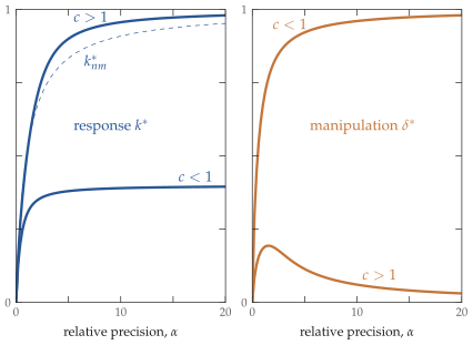
Citizens’ equilibrium response \(k^*\) (left panel) and politician’s equilibrium manipulation \(\delta^*\) (right panel) as functions of the relative precision \(\alpha\) for various levels of the costs of manipulation \(c\). The citizens’ \(k^*\) is increasing in \(\alpha\) and asymptotes to \(\min[c,1]\) as \(\alpha \rightarrow \infty\). If \(c<1\) then in equilibrium the politician’s marginal benefit of manipulation is increasing in \(k\) so \(\delta^*\) increases with \(k^*\) as \(\alpha\) rises and asymptotes to one as \(k^*\rightarrow c\). If \(c>1\) then for high enough \(\alpha\) we have \(k^*>\hat{k}(c)\) so that the politician’s marginal benefit of manipulation is decreasing in \(k\) so that \(\delta^*\) starts to decrease and asymptotes to zero as \(k^*\rightarrow 1\).

Open this figure on its own page

We illustrate this result in Figure 3 which shows the citizens’ equilibrium response \(k^*\) (left panel) and politician’s equilibrium manipulation \(\delta^*\) (right panel) as functions of the costs of manipulation \(c\) for the case of low \(\alpha<1\) and high \(\alpha>1\). If \(\alpha<1\) then we know from Lemma 1 that the precision effect dominates so that the citizens’ \(k(\delta;\alpha)\) curve is decreasing and so \(k^*\) and \(\delta^*\) move in opposite directions following a change in \(c\). Alternatively, if \(\alpha>1\), then the level of \(\delta^*\) matters, and this depends on the level of \(c\). If \(c\) is low, then \(\delta^*\) will be high so the precision effects continues to dominate meaning that \(k^*\) and \(\delta^*\) move in opposite directions following a change in \(c\). But if \(c\) is high enough to make \(\delta^*\) low, then the correlation effect will dominate and \(k^*\) and \(\delta^*\) will move in the same direction following a change in \(c\).

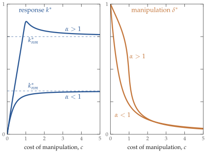
Citizens’ equilibrium response \(k^*\) (left panel) and politician’s equilibrium manipulation \(\delta^*\) (right panel) as functions of the politician’s costs of manipulation \(c\) for various levels of the relative precision \(\alpha\). The politician’s \(\delta^*\) is decreasing in \(c\) and asymptotes to zero as \(c\rightarrow \infty\). If \(\alpha<1\), the precision effect dominates so that as \(\delta^*\) decreases the citizens’ \(k^*\) increases and asymptotes to \(k^*_{nm}\) from below as \(c\rightarrow\infty\). If \(\alpha>1\) then for high enough \(c\) we have \(\delta^*<\hat{\delta}(\alpha)\) so that the correlation effect begins to dominate at which point \(k^*\) starts to decrease and asymptotes to \(k^*_{nm}\) from above as \(c\rightarrow \infty\).

Open this figure on its own page

3.6 “Regime changes” In the Amount of Manipulation

Intuitively, the politician’s equilibrium manipulation \(\delta^*\) is always decreasing in the costs of manipulation \(c\). Perhaps more surprisingly, however, it turns out that the equilibrium manipulation \(\delta^*\) can also feature a jump at the threshold \(c=1\). Because of this, even small changes in the costs of manipulation can trigger “regime changes” in the amount of manipulation. In particular, near the threshold \(c=1\) the size of the change in manipulation is given by:

In particular, when \(c\) is close to the critical threshold \(c=1\), there will be an especially large reduction in manipulation when the relative precision \(\alpha:=\alpha_x/\alpha_z\) is high, i.e., when the intrinsic signal precision \(\alpha_x\) is high or the prior precision \(\alpha_z\) is low. This large reduction in manipulation close to \(c=1\) is most stark when \(\alpha>4\). In this case, a small increase from \(c=1-\varepsilon\) to \(c=1+\varepsilon\) will cause the amount of manipulation to jump from \(\overline{\delta}(\alpha)>1/2\) down to \(\underline{\delta}(\alpha)<1/2\). In the limit as \(\alpha\rightarrow\infty\) we have \(\overline{\delta}(\alpha)\rightarrow 1\) and \(\underline{\delta}(\alpha)\rightarrow 0\) so that the manipulation jumps from \(\delta^*=1\) (full manipulation) to \(\delta^*=0\) (no manipulation). We illustrate this in Figure 4 which shows the equilibrium manipulation \(\delta^*\) as a function of \(c\) for \(\alpha<4\) (lighter), \(\alpha=4\), and \(\alpha>4\) (darker). For \(\alpha<4\) the manipulation is smoothly decreasing in \(c\) with a mild slope at \(c=1\). For \(\alpha=4\) the derivative at \(c=1\) is very steep. For \(\alpha>4\) the manipulation jumps from \(\overline{\delta}(\alpha)>1/2\) to \(\underline{\delta}(\alpha)<1/2\) at \(c=1\).

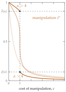
Equilibrium manipulation \(\delta^*\) as a function of \(c\) for \(\alpha<4\) (lighter), \(\alpha=4\) and \(\alpha>4\) (darker). For \(\alpha\leq 4\), the manipulation \(\delta^*\) is continuous in \(c\). But for \(\alpha>4\) the manipulation jumps discontinuously at \(c=1\). In the limit as \(\alpha\rightarrow\infty\) the boundaries \(\underline{\delta}(\alpha)\rightarrow 0^+\) and \(\overline{\delta}(\alpha)\rightarrow 1^+\) so that the manipulation jumps by the maximum amount, from \(\delta^*=0\) if \(c<1\) to \(\delta^*=1\) if \(c>1\).

Open this figure on its own page

Intuition for large changes in manipulation near \(c=1\). To understand this result, recall from (22) that the politician’s optimal manipulation can be written \[\tag{28} \delta(k)=\operatornamewithlimits{argmax}_{\delta\in[0,1]} \, [\, B(\delta,k)-C(\delta)\,]\] where \(B(\delta,k)\) denotes the politician’s benefit from manipulation, which is increasing in the distance between the citizens’ average action \(A\) and the true \(\theta\), and where \(C(\delta)\) denotes the costs of manipulation, which is increasing in the distance between the manipulated average signal \(y\) and the true \(\theta\), with coefficient \(c\). As the relative precision \(\alpha\) increases, the citizens become more responsive to their signals, i.e., \(k\) increases, so that the citizens’ average action \(A\) becomes close to the average signal, \(A\rightarrow y\). In short, the politician’s benefit from manipulation is increasingly similar to his/her costs of manipulation, differing only by the magnitude of \(c\). Small changes in \(c\) near \(c=1\) can thus lead to large changes in the amount of manipulation when \(\alpha\) is high.

Now that we have a complete understanding of the comparative statics of the model, we can turn to our main interest, the welfare effects of a social media revolution, a simultaneous increase in the intrinsic precision \(\alpha_x\) and decrease in the costs of manipulation \(c\).

4 Welfare Effects of the Social Media Revolution

In this section we use our model to interpret the social media revolution. In particular, we argue that the social media revolution makes possible the kind of “regime change” in the amount of manipulation highlighted in Proposition 2 above. Whether a social media revolution is welfare-improving for the citizens then depends on whether the costs of manipulation can be kept above the critical threshold \(c=1\). If this can be achieved, the social media revolution will decrease manipulation and make the citizens better off. But if instead the costs of manipulation fall below the critical threshold, then the social media revolution will lead to a large increase in manipulation, preventing the benefits of intrinsically precise information from passing through to the citizens, thereby making the citizens worse off.

Pessimism and optimism about new media technologies. The strategic use of information manipulation, whether it be blatant propaganda or more subtle forms of misdirection and obfuscation, is a timeless feature of human communication. The role that new technologies play in either facilitating or impeding this information manipulation is widely debated and optimism or pessimism on this issue seems to fluctuate as new technologies develop. For example, in the postwar era a pessimistic view emphasized the close connections between mass media technologies like print media, radio and cinema and the immersive propaganda of totalitarian regimes (e.g., Friedrich and Brzezinski 1965; Arendt 1973; Zeman 1973). But in the 1990s and 2000s, a more optimistic view stressed the potential benefits of the internet and other, relatively more decentralized methods of communication, in undermining attempts to control information. This optimism seems to have reached its zenith during the “Arab Spring” protests against autocratic regimes in Tunisia, Egypt, Libya and elsewhere beginning in 2010. But increasingly the dominance of social media like Facebook and Twitter has led to renewed pessimism (e.g., Morozov 2011). In particular, the apparent role of such platforms in facilitating the spread of misleading information during major political events, like the 2016 UK Brexit referendum and the 2016 US presidential election, has led to newly intense scrutiny of social media technologies (e.g., Faris et al. 2017).

The challenge of social media As emphasized by Bruns and Highfield (2012) and Allcott and Gentzkow (2017), social media technologies have two features that are particularly relevant. First, they have low barriers to entry and it has become increasingly easy to commercialize social media content through tools like Google and Facebook advertising. This has lead to a proliferation of new entrants that have been able to establish a viable market for their content. Second, social media technologies have significantly reduced the costs of collecting, reporting and disseminating information, and have thus lead to a rapidly expanded role of blogging and amateur journalism in the media industry. As emphasized by Fielder (2009) and Ward (2011), these new sources of information are not all subject to the same standards of accountability as traditional journalism. Moreover, the new social media technologies also mean that citizens consume much of their media content in a feed that both blurs distinctions between reliable and unreliable sources of information and also makes it easy for all kinds of news, real and fake, to “go viral” — to be rapidly retweeted or shared.

In the context of our model, we view these two features of social media as simultaneously (i) increasing the underlying, intrinsic signal precision \(\alpha_x\), but (ii) decreasing the costs of manipulation \(c\). Social media technologies facilitate the entry of new media outlets and amateur journalists, which leads to a large increase in the news and information collected and disseminated. Absent manipulation, this would mean more signals and hence an increase in the intrinsic quality of information.⁸ But the entry of low-accountability media outlets and amateur journalism and the technological ease with which stories can go viral, diffusing rapidly in the population, also bring new tools for a politician to use spin and misdirection to undermine the credibility of the information reported in the media. In this sense, the rise of social media creates a new more decentralized and flexible cost structure for information manipulation. According to the Oxford Internet Institute’s Global Inventory of Organized Social Media Manipulation (Bradshaw and Howard 2019), evidence of organized social media manipulation campaigns by governments and political parties has been found in 70 countries in 2019, up from 48 countries in 2018 and 28 countries in 2017. Presumably, this rapid increase in uptake largely reflects a reduction in the costs of manipulation \(c\) rather than an increase in the demand for manipulation.

In short, the simultaneous change in \(\alpha_x\) and \(c\) creates a tension. We now turn to analyze the net effect of this tension.

4.1 Citizens’ Welfare

We begin with the welfare effects of the social media revolution on the citizens. In particular, we show that, when the politician can manipulate information, an increase in the intrinsic precision \(\alpha_x\) that would absent manipulation, make the citizens better off, can end up making them worse off instead.

Citizens’ indirect utility. We measure the citizens’ welfare in the following way. To begin with, let \(l(\delta)\) denote the loss function \[\tag{29} l(\delta):=\min_{k\in[0,1]}\, L(k,\delta)\] where \(L(k,\delta)\) denotes the citizens’ ex ante expected loss, i.e., the expectation of \(\int_0^1\,(a_i-\theta)^{2}\,di\) with respect to the prior that \(\theta\) is normally distributed with mean \(z\) and precision \(\alpha_z\), if they choose \(k\) when the politician has manipulation \(\delta\). This works out to be \[\tag{30} L(k,\delta) = \frac{1}{\alpha_z} B(\delta,k) + \frac{1}{\alpha_x}k^2\] where again \(B(\delta,k):=(k\delta+1-k)^2\) denotes the politician’s benefit from manipulation. Evaluating at the citizens’ best response \(k(\delta)\) and collecting terms gives \[\tag{31} l(\delta) = L(k(\delta),\delta) = \frac{1}{\alpha_x}\,\left(\frac{k(\delta)}{1-\delta}\right) = \left(\frac{1}{1+\alpha(1-\delta)^2}\right)\,\frac{1}{\alpha_z}\] The prior precision \(\alpha_z\) simply scales the whole loss. To simplify the discussion, we measure payoffs for the citizens by the term \(u=\alpha(1-\delta)^2\) which depends only on the relative precision \(\alpha:=\alpha_x/\alpha_z\) and the costs of manipulation \(c\), and has the orientation of a utility function in the sense that a higher \(u\) indicates better outcomes for the citizens. More precisely, let \(u^*(\alpha,c)\) denote the citizens’ indirect utility evaluated at the equilibrium manipulation \[\tag{32} u^*(\alpha,c) := \alpha (1-\delta^*(\alpha,c))^2\] This indirect utility is a natural measure of welfare outcomes for the citizens. Recall that the synthetic signal \(\hat{x}_i\) used in the citizens’ signal extraction problem has precision \(\alpha_x (1-\delta)^2\). So \(u^*(\alpha,c)\) is the equilibrium precision of the synthetic signal scaled by the prior precision \(\alpha_z\). Absent manipulation, we have \(u^*_{nm}:=u^*(\alpha,\infty)=\alpha\) and an increase in the precision of the signal passes through one-to-one to welfare. But with manipulation there is incomplete passthrough and indeed an increase in \(\alpha\) need not be welfare-improving for the citizens.

Social media revolution can make citizens worse off. Our main result here is:

To understand this result, observe that an increase in \(\alpha\) has both a direct effect on the citizens’ utility and an indirect effect through the politician’s manipulation \(\delta^*(\alpha,c)\). In turn, from Lemma 3 above, we know that the indirect effect of \(\alpha\) through the politician’s \(\delta^*\) depends on the magnitude of \(c\). In particular, if the costs of manipulation are relatively high, \(c>1\), then \(\delta^*\) is decreasing in \(\alpha\) and so the direct and indirect effects reinforce one another. The citizens’ loss is thus unambiguously increasing in \(\alpha\), as in part (i) of the proposition. But if the costs of manipulation are relatively low, \(c<1\), then \(\delta^*\) is increasing in \(\alpha\) when \(\alpha\) is sufficiently high and so the indirect effect works against the direct effect. We show in the Appendix that if \(c<1\) there is a finite critical point \(\alpha^{*}\) such that the indirect effect via the politician’s manipulation \(\delta^*\) dominates if and only if \(\alpha>\alpha^{*}\), as in part (ii) of the proposition. Finally, since the politician’s manipulation \(\delta^*\) is strictly decreasing in the costs of manipulation \(c\), the citizens’ utility is strictly increasing in \(c\). Moreover, if \(\alpha>4\) the citizens’ utility has a jump discontinuity inherited from the jump in manipulation characterized in Proposition 2 above.

We illustrate this result in Figure 5 which shows the citizens’ utility \(u^*\) as a function of \(\alpha\) for \(c>1\) and \(c<1\). For reference we also show the citizens’ utility without manipulation \(u_{nm}^*=\alpha\), the dashed \(45\)-degree line. With manipulation the citizens are always worse off, \(u^*<u_{nm}^*\). If \(c>1\) the citizens’ utility is strictly increasing in \(\alpha\). If \(c<1\) the citizens’ utility is first increasing, reaches an interior maximum at \(\alpha=\alpha^*\), then decreases. For \(\alpha>4\) the citizens’ utility has a jump discontinuity in \(c\) at the critical threshold \(c=1\). In this figure, this is seen in the relatively large change in \(u^*\) from \(c>1\) to \(c<1\) when \(\alpha>4\).

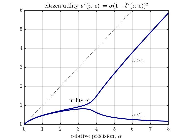
Citizens’ utility \(u^*\) as a function of \(\alpha\) for \(c>1\) and \(c<1\). For \(c>1\) the citizens’ utility is strictly increasing in \(\alpha\). For \(c<1\) the citizens’ utility reaches an interior maximum at \(\alpha=\alpha^*\) and then decreases \(u^*\rightarrow 0\) as \(\alpha\rightarrow\infty\). As a function of \(c\), the citizens’ utility inherits the jump discontinuity in \(\delta^*\) at \(c=1\).

Open this figure on its own page

Asymptotic welfare. The citizens’ welfare outcomes are seen most starkly in the limits:

Regardless of \(c\), the citizens’ utility starts at \(u^*(0,c)=0\). If \(c>1\) the citizens’ utility is strictly increasing and since in this case the politician’s manipulation \(\delta^*\rightarrow 0\) as \(\alpha\rightarrow\infty\) we have \(u^*/\alpha\rightarrow 1\). Recall that absent manipulation, the citizens have utility \(u_{nm}^*=\alpha\), so this is equivalently \(u^*/u_{nm}^*\rightarrow 1\). So for \(c>1\) and \(\alpha\) large the manipulation is essentially shrugged off and the further increases in \(\alpha\) pass through one-for-one to the citizens. But if \(c<1\) the citizens’ utility reaches an interior maximum and then declines \(u^*\rightarrow 0\) as \(\alpha\rightarrow\infty\), the same utility they would have if \(\alpha=0\). In this scenario, even though the intrinsic precision of their signals is extremely high, the citizens have the same utility as if they had no information other than their prior.

4.2 Two Kinds of Social Media Revolutions

Recall that we interpret the social media revolution as simultaneously increasing \(\alpha\) and decreasing \(c\). Given this, the preceding discussion implies that there are really two kinds of social media revolutions, with quite different implications. To be concrete, suppose that initially the economy has relatively high costs of manipulation \(c_0>1\) and that following the social media revolution these costs are \(c_1<c_0\). And suppose that the social media revolution increases the precision from \(\alpha_0\) to \(\alpha_1>\alpha_0\). The key consideration is whether the decrease in \(c\) is large enough to push the costs of manipulation below the critical threshold \(c=1\).

High manipulation regime. If we get to \(c_1<1\) when the intrinsic precision \(\alpha\) is high, then the economy will end up in a high manipulation regime where the citizens must be worse off on net. In particular:

That is, if the initial precision \(\alpha_0\geq \alpha^{**}(c_0,c_1)\), then the initial utility \(u^*(\alpha_0,c_0)\) with the high costs of manipulation \(c_0>1\) exceeds the utility \(u^*(\alpha_1,c_1)\) with the low costs of manipulation \(c_1<1\) regardless of the subsequent precision \(\alpha_1\).

To visualize this, consider Figure 5 above and fix \(c_1<1\). Maximizing over \(\alpha\), the highest utility the citizens can obtain is \(u^*(\alpha^*(c_1),c_1)\). Now fix \(c_0>1\) for which \(u^*(\alpha,c_0)\) is strictly increasing in \(\alpha\). Then let \(\alpha^{**}(c_0,c_1)\) denote the unique solution to \[\tag{34} u^*(\alpha^{**},c_0) = u^*(\alpha^*(c_1),c_1)),\qquad c_0>1>c_1\] Since \(u^*(\alpha,c_0)\) is strictly increasing in \(\alpha\), the level of utility \(u^*(\alpha_0,c_0)\) is unobtainable by \(u^*(\alpha,c_1)\) for any \(\alpha_0>\alpha^{**}(c_0,c_1)\). One might have thought that, although the decrease in the costs of manipulation \(c_0>1>c_1\) hurts the citizens, there could be a compensating change in \(\alpha\) that is enough to offset this and leave the citizens no worse off. This result establishes that such compensation is available only if the initial precision \(\alpha_0\) is sufficiently low. For \(\alpha_0> \alpha^{**}(c_0,c_1)\) there is no change in \(\alpha\) that can compensate for the decrease in the costs of manipulation \(c_0>1>c_1\).

This result is driven by the fact that when \(c<1\) the politician’s manipulation \(\delta\) is increasing in the citizens’ response \(k\) so that as \(\alpha\) increases and the citizens respond more to their signals, the politician in turn also increases the amount of manipulation. Because of this, the equilibrium information content of the citizens’ signals falls even though the underlying, intrinsic precision of their signals is rising. Indeed, for \(c<1\) as \(\alpha\rightarrow\infty\), the citizens’ utility is driven \(u^*\rightarrow 0\), i.e., the same utility the citizens would have if \(\alpha=0\). In this sense, the manipulation causes the citizens to lose all the potential benefits from high \(\alpha\).

Low manipulation regime. Alternatively, if the costs of manipulation do not fall too much, i.e., if we keep \(c_1>1\), then the economy will end up in a low manipulation regime. In this low manipulation regime, an increase in \(\alpha\) may be enough to compensate for the fall in \(c\) and the citizens may be better off on net. To see the net effect, we plot the indifference curves of \(u^*(\alpha,c)\) in Figure 6 with warmer colors indicating higher utility. A social media revolution that moves us towards warmer colors has a net positive effect on citizens’ utility. Notice that no other parameter enters the utility \(u^*(\alpha,c)\), so the plot shown here is a fully global characterization. One can simply read off this figure whether utility on net increases or decreases for every possible change in \(\alpha\) and \(c\).

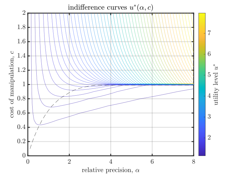
Citizens’ indifference curves \(u^*(\alpha,c)\) with warmer colors indicating higher utility. For \(c>1\), higher \(\alpha\) increases the citizens’ utility. For \(c<1\) and \(\alpha>\alpha^*(c)\), higher \(\alpha\) decreases the citizens’ utility. For \(\alpha>4\) the citizens’ utility jumps discontinuously at the critical threshold \(c=1\). The levels of utility with \(\alpha>4\) and \(c>1\) cannot be reached from any \(c<1\).

Open this figure on its own page

In the low manipulation regime, the outcomes are driven by the fact that when \(c>1\) the politician’s manipulation \(\delta\) is decreasing in the citizens’ response \(k\) so that as \(\alpha\) increases and the citizens respond more to their signals, the politician manipulates less and less. In this sense, keeping \(c>1\) is sufficient to ensure the citizens benefit from high \(\alpha\).

In other words, even relatively small changes in the conduct of social media platforms that make it harder to manipulate information may be surprisingly effective. Such changes could come from greater internal efforts to regulate social media content, better technologies that help distinguish reliable information sources from less reliable ones, more rigorous scrutiny of politicians’ speeches and interviews, etc.

4.3 Politician’s Welfare

We now turn to the welfare effects of a social media revolution on the politician.

Politician’s payoff. Let \(v(k)\) denote the politician’s value function \[\tag{35} v(k) := \max_{\delta \in[0,1]}\, V(\delta,k)\] where \(V(\delta,k)\) denotes the politician’s ex-ante expected payoff if they choose manipulation \(\delta\) when the citizens have response coefficient \(k\). From (22) this works out to be \[\tag{36} V(\delta,k) = \frac{1}{\alpha_z} (B(\delta,k) - C(\delta)) + \frac{1}{\alpha_x}k^2\] where again \(B(\delta,k):=(k\delta+1-k)^2\) and \(C(\delta):=c\delta^2\). Evaluating \(V(\delta,k)\) at the politician’s best response \(\delta(k)\) and collecting terms gives the value function \[\tag{37} v(k) = V(\delta(k),k) = \left((1-k)^2\left(\frac{c}{c-k^2}\right)+\frac{1}{\alpha}k^2 \right)\,\frac{1}{\alpha_z}\] As with the citizens, the prior precision \(\alpha_z\) scales the whole payoff. It then simplifies the discussion to focus on the normalized payoff \(v^*:=v(k^*)\alpha_z\) which depends only on the relative precision \(\alpha:=\alpha_x/\alpha_z\) and the costs of manipulation \(c\). Write this as \(v^*(\alpha,c)\). Absent manipulation, the politician’s payoff is \(v^*_{nm}(\alpha):=v^*(\alpha,\infty)\).

Social media revolution can make politician better off. Our main result here is:

To understand this result, notice that this payoff \(v^*:=v(k^*)\alpha_z\) depends on \(\alpha\) and \(c\) both directly and indirectly via the equilibrium response \(k^*(\alpha,c)\). The effect of a change in \(\alpha\) is proportional to \[\tag{39} \frac{\partial v(k^*;\alpha)}{\partial \alpha} + v'(k^*)\frac{\partial k^*}{\partial \alpha}\] The first term is the direct effect and is negative according to (37). The second term is the indirect equilibrium effect through the citizens’ response coefficient \(k^*\). Since the politician takes \(k^*\) as given, we cannot simply invoke the envelope theorem to ignore this indirect equilibrium effect. But for our benchmark model it turns out that indeed \(v'(k^*)=0\) so that nonetheless this indirect effect can be ignored. Consequently \(v^*\) is strictly decreasing in \(\alpha\).

A similar argument applies to the effect of a change in \(c\). From (37) the direct effect of higher costs of manipulation \(c\) is to decrease the politician’s payoff \(v^*\) and since for our benchmark model \(v'(k^*)=0\) this is the only effect. So for any fixed \(\alpha\), we have that \(v^*(\alpha,c)>v^*(\alpha,\infty)=:v^*_{nm}(\alpha)\). In this sense, the politician always benefits from their ability to manipulate information. If given the option to credibly commit to not manipulate information they would never take that option.

The fact that \(v'(k^*)=0\) simplifies this calculation greatly. This is a consequence of the fact that the politician’s objective is essentially the mirror image of the citizens’ objective. While the politician takes \(k\) as given so we cannot invoke the politician’s optimality conditions to set \(v'(k^*)=0\), the citizens do not take \(k\) as given and we can invoke the citizens’ optimality conditions to set \(v'(k^*)=0\). This suggests that \(v'(k^*)=0\) is a somewhat knife-edge result. Once the politician’s objective and the citizens’ objective are no longer mirror images of each other we cannot invoke this argument and we will find that \(v'(k^*)\) need not be zero.⁹

In Figure 7, we illustrate the politician’s payoff \(v^*\) as a function of \(\alpha\) for \(c>1\) and \(c<1\). For reference we also show the politician’s payoff without manipulation \(v_{nm}^*\), the dashed black line. Regardless of \(c\), the politician’s payoff starts at \(v^*(0,c)=1\). For each \(c\), the politician’s payoff is strictly decreasing in \(\alpha\). For each \(\alpha\), the politician’s payoff is strictly decreasing in \(c\). In particular, \(v^*>v^*_{nm}\) so that the politician is always better off when they can manipulate information. For large \(\alpha\) the politician’s payoff crucially depends on the costs of manipulation \(c\). If the costs of manipulation are relatively high, \(c>1\), then in the limit as \(\alpha\rightarrow\infty\) we have \(v^*\rightarrow 0\) and \(v^*_{nm}\rightarrow 0\) so that in this case the politician’s gain from manipulation \(v^*-v^*_{nm}\) becomes negligible. But if the costs of manipulation are relatively low, \(c<1\), then in the limit as \(\alpha\rightarrow\infty\) we have \(v^*\rightarrow 1-c\). In other words, if \(c<1\) the politician’s payoff is bounded below by \(1-c\). Since the politician’s payoff absent manipulation \(v_{nm}^*\rightarrow 0\), the politician’s asymptotic gain from manipulation in this case is also \(1-c\) which is then large if in addition the costs of manipulation are low.

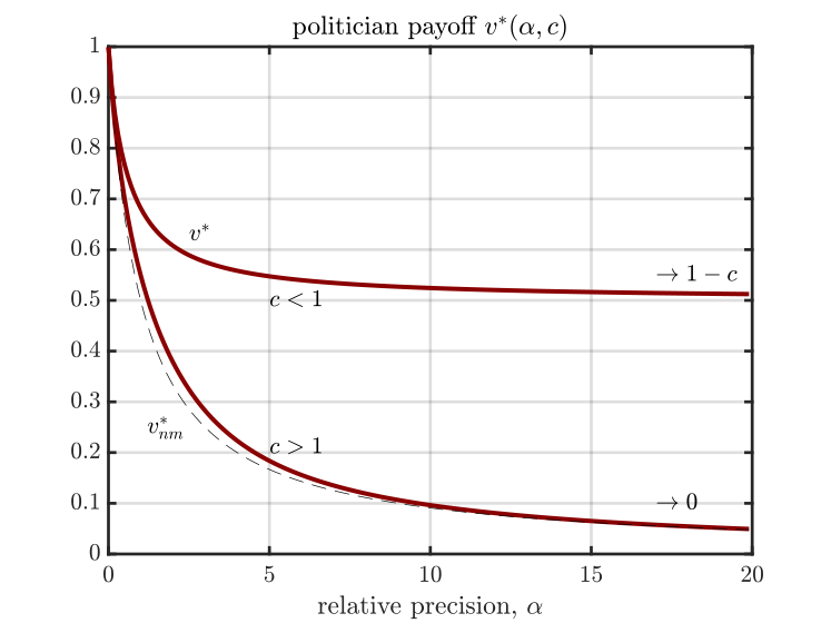
Politician’s payoff \(v^*\) as a function of \(\alpha\) for \(c>1\) and \(c<1\). The politician’s payoff is strictly decreasing in \(\alpha\) and \(c\). Hence \(v^*>v_{nm}^*\). For \(c>1\) the politician’s payoff \(v^*\rightarrow 0\) as \(\alpha\rightarrow\infty\). For \(c<1\) the politician’s payoff \(v^*\rightarrow 1-c\) as \(\alpha\rightarrow\infty\). In this sense the politician’s gain from manipulation \(v^*-v_{nm}^*\) is large when \(\alpha\) is large and \(c\) is small.

Open this figure on its own page

In particular, in the cheap talk limit \(c\rightarrow 0\), the politician’s payoff is kept at \(v^*=1\) independent of \(\alpha\). In this case, the politician’s manipulation \(\delta^*\rightarrow 1\) so that in equilibrium the citizens have completely uninformative signals regardless of the level of \(\alpha\).

High and low manipulation regimes revisited. Now recall that we interpret the social media revolution as a simultaneous increase in \(\alpha\) from \(\alpha_0\) to \(\alpha_1\) and decrease in \(c\) from \(c_0\) to \(c_1\). As with the citizens, the key consideration is whether the decrease in \(c\) is large enough to push the costs of manipulation below the critical threshold \(c = 1\). If the decrease in the costs of manipulation is large enough, \(c_0>1>c_1\), then we enter a high manipulation regime where the amount of manipulation increases substantially and the politician’s payoff is bounded below by \(1-c_1\). Then for any initial precision \(\alpha_0\) such that \(v^*(\alpha_0,c_0)<1-c_1\) the social media revolution overall makes the politician better off. That is, although the increase from \(\alpha_0\) to \(\alpha_1\) reduces the politician’s payoff, this effect is not enough to offset the politician’s gain from the relatively large reduction in the costs of manipulation. Alternatively if the decrease in the costs of manipulation is not too large, \(c_0>c_1>1\), then we enter a low manipulation regime where any \(\alpha_1\) such that \(v^*(\alpha_1,c_1)<v^*(\alpha_0,c_0)\) is sufficient to ensure that the social media revolution overall makes the politician worse off.

In short, we find that overall the social media revolution can trigger a kind of “regime change” in the amount of manipulation that not just dampens the citizens’ benefit from an increase in the precision \(\alpha\) but actually makes them worse off overall and at the same time makes the politician better off. We next turn to a discussion of the robustness of this result.

5 Extensions

In this section we discuss two extensions of our benchmark model. Section 5.1 outlines a version of the model where citizens obtain their information from the media, a collection of journalists with preferences that may not perfectly reflect the preferences of the citizens. Section 5.2 returns to the basic setup with just the citizens but adds two other features: (i) heterogeneous priors, and (ii) endows the politician with the ability to directly manipulate the signal variance, not just the signal mean. The full details of these extensions are given in our Supplementary Online Appendix.

5.1 Active Media

Setup. Suppose that on the receiving end of the politician’s manipulation is a set of journalists \(j\in[0,1]\). Each journalist chooses a report \(a_j\) that balances (i) a desire to accurately report the true \(\theta\) with (ii) the way their individual report \(a_j\) fits with the average report \(A:=\int_0^1 a_j \,dj\). In particular, each journalist chooses \(a_j\) to minimize the expected value of the quadratic loss \[\tag{40} (1-\lambda)(a_j-\theta)^2 + \lambda (a_j-A)^2,\qquad \lambda<1\] where the parameter \(\lambda\) governs the strategic interactions among journalists. If \(\lambda<0\) then each journalist’s report \(a_j\) and the average report \(A\) are strategic substitutes. In this case each journalist wants their report \(a_j\) to be consistent with \(\theta\) but also wants to make their \(a_j\) stand out from the crowd, differing from \(A\). By contrast if \(\lambda\in(0,1)\) then each journalist’s report \(a_j\) and the average report \(A\) are strategic complements. In this case, each journalist wants their report \(a_j\) to be consistent both with \(\theta\) and with \(A\). We suppose that the reports are consumed by citizens who value only how accurately these reports reflect the truth, as in the benchmark model. The interests of the citizens and the journalists are perfectly aligned in the special case \(\lambda=0\).

As in the benchmark model, the journalists’ have common priors \(\theta\sim N(0,\alpha_z^{-1})\) and signals \(x_j\sim N(y,\alpha_x^{-1})\) where the politician chooses the signal mean \(y\) at cost \(c(y-\theta)^2\). The optimal action of a journalist with signal \(x_j\) is \[\tag{41} a(x_j) = (1-\lambda)\mathbb{E}[\theta\,|\,x_j] + \lambda \mathbb{E}[A(\theta)\,|\,x_j]\]

Equilibrium. We focus on a symmetric equilibrium in linear strategies \(a(x_j)=k x_j + (1-k)z\) for some coefficient \(k\) to be determined. This implies \(A(\theta)=ky(\theta)+(1-k)z\). The politician again has strategy \(y(\theta)=(1-\delta)\theta+\delta z\) with manipulation coefficient \(\delta(k)=(k-k^2)/(c-k^2)\). Solving the journalists’ signal extraction problem and matching coefficients we find that the journalists’ response coefficient is given by \[\tag{42} k(\delta) = \frac{(1-\delta)\alpha}{(1-\delta)^2 \alpha+1},\qquad \alpha:=(1-\lambda)\frac{\alpha_x}{\alpha_z}\] This is the same as in the benchmark model but the composite precision parameter \(\alpha\) now contains a term \((1-\lambda)\) that increases the relative weight on the idiosyncratic signals if the journalists’ actions are strategic substitutes and increases the relative weight on the common prior if the journalists’ actions are strategic complements. Other than this, the equilibrium is determined by the intersection of the \(k(\delta;\alpha)\) and \(\delta(k;c)\) curves, as in our benchmark model.

Welfare results. Relative to our benchmark model, we obtain two new welfare results. First, we find that if the strategic interactions among the journalists are sufficiently strong, \(|\lambda|>1/2\), the manipulation may backfire on the politician. In particular if either (i) \(\lambda>1/2\) and \(c>1\) and \(\alpha_x\) is sufficiently high, or (ii) \(\lambda<-1/2\), \(c<1\) and \(\alpha_x\) is sufficiently low, the manipulation backfires, \(v^*<v_{nm}^*\). In either of these scenarios, the politician would be better off if they could credibly commit to not use their manipulation technology at all, i.e., they would be better off if \(c=+\infty\) (hence we also find that a reduction in \(c\) need not make the politician better off). That said, the politician still does benefit from manipulation when \(c\) is low and \(\alpha_x\) is sufficiently high. In other words, a social media revolution that decreases \(c\) by enough and increases \(\alpha_x\) by enough will make the politician better off, as in our benchmark model.

Second, we find that while manipulation of the journalists’ signals generally makes the citizens worse off, there is now a narrow set of circumstances where the manipulation is actually in the citizens’ interest. If the journalists’ actions are sufficiently strong strategic substitutes \(\lambda<-1\) and the intrinsic signal precision \(\alpha_x\) is sufficiently low, then absent manipulation the journalists will seek to strongly differentiate themselves from one another, too much so from the citizens’ point of view. The politician’s manipulation then dampens the journalists’ response to their signals, which is beneficial to the citizens. But of course a social media revolution that makes \(\alpha_x\) high is working at the other end of the spectrum and does not have this beneficial effect.

5.2 Heterogeneous Priors and Manipulation of the Signal Variance

We now turn to another extension of our benchmark model where we allow the citizens to have heterogeneous priors and allow the politician to manipulate the signal variance.

Setup. Suppose citizens have priors \(z_i=z+\eta_i\) that are the sum of a common component \(z=\theta+\varepsilon_z\) with \(\varepsilon_z\sim N(0,\sigma_z^2)\) and an idiosyncratic component \(\eta_i\sim N(0,\sigma_{\eta}^2)\). The citizens have their usual noisy signal \(x_i=y+\varepsilon_i\) but now the signal variance is \(\gamma \sigma_x^2\) where the variance manipulation factor \(\gamma\) is chosen by the politician subject to a quadratic cost \(c_{\gamma} (\gamma-1)^2\). We again consider linear strategies for the citizens \(a(x_i,z_i)= kx_i + (1-k)z_i\). The politician’s best response for the variance manipulation works out to be \[\tag{43} \gamma(k) = 1 + \frac{\sigma_x^2}{2c_\gamma} k^2\] while the politician’s best response for the signal mean is as before \[\tag{44} y = (1-\delta) \theta + \delta z,\qquad \delta(k) = \frac{k-k^2}{c-k^2}\] and the citizens’ best response to the politician’s manipulation works out to be \[\tag{45} k(\delta,\gamma) = \frac{(1-\delta)\sigma_z^2 + \sigma_{\eta}^2}{(1-\delta)^2 \sigma_z^2 + \sigma_{\eta}^2 + \gamma\sigma_x^2}\] Our benchmark model is nested as the special case where both (i) \(c_{\gamma}\rightarrow\infty\), so that the politician always chooses \(\gamma=1\), i.e., the signal variance is just the exogenous \(\sigma_x^2\), and (ii) \(\sigma_{\eta}^2=0\) so that there is no prior dispersion.

Equilibrium. An equilibrium is a triple \(k^*,\delta^*,\gamma^*\) simultaneously satisfying conditions (43), (44) and (45). As in the benchmark model, there is a unique (linear) equilibrium.

Results. This extended model leads to two new results. First, we show that a version of our key equilibrium result Proposition 2, i.e., the result that leads to the welfare implications in our benchmark model, continues to hold in this extended model. In particular, we find that \(\delta^*\) jumps discontinuously at \(c=1\) if the intrinsic signal variance \(\sigma_x^2\) is below a critical threshold (i.e., the intrinsic signal precision \(\alpha_x=1/\sigma_x^2\) is above a critical threshold). Moreover, the size of the jump in \(\delta^*\) is decreasing in \(\sigma_x^2\) (i.e., increasing in the precision \(\alpha_x=1/\sigma_x^2\)) but is independent of the amount of prior dispersion \(\sigma^2_{\eta}\).

Second, we show that the equilibrium signal variance \(\sigma_x^{2\,*}=\gamma^* \sigma_x^2\) is (i) increasing in the intrinsic signal variance \(\sigma_x^2\) and (ii) is increasing in the prior dispersion \(\sigma_{\eta}^2\). This means that the increase in signal precision that we exogenously assumed in our benchmark model can now be interpreted as an equilibrium outcome in this extended model. A reduction in the intrinsic signal variance \(\sigma_x^2\) or a reduction in the prior dispersion \(\sigma_{\eta}^2\) both drive down the equilibrium signal variance \(\sigma_x^{2\,*}\) thereby giving citizens better information.

To understand the second result, observe from equation (43) that the politician’s variance manipulation \(\gamma\) is increasing in both \(\sigma_x^2\) and the citizens’ response \(k\). In equilibrium, the citizens’ response \(k^*\) is decreasing in \(\sigma_x^2\). So an increase in \(\sigma_x^2\) has both the direct effect of increasing the amount of variance manipulation and an indirect effect via \(k^*\) of decreasing the amount of variance manipulation. It turns out that the direct effect always dominates the indirect effect. In equilibrium, the citizens’ response \(k^*\) is also increasing in the prior dispersion \(\sigma_{\eta}^2\). Hence, a higher prior dispersion \(\sigma_{\eta}^2\) that increases \(k^*\) also increases the amount of variance manipulation \(\gamma^*\).

6 Conclusions

We argue that even small changes in social media platforms that make it harder for misinformation to spread may play an important role in ensuring that society benefits from social media technologies overall. We arrive at this conclusion by developing a model of information manipulation with one politician and many imperfectly informed citizens. The politician manipulates information in an effort to prevent the citizens from making informed decisions. The citizens are rational and internalize the politician’s incentives. In equilibrium the citizens’ information is unbiased but endogenously noisy, making the citizens worse off and the politician better off than they would be if manipulation was impossible.

We interpret the social media revolution as a shock that simultaneously changes two features of the information environment. First, these new technologies have led to new sources of information, both in the form of new media outlets and in the form of blogging and amateur journalism, thereby increasing the underlying, intrinsic precision of the information available to the citizens. Second, these new sources of information are not all subject to the same standards of accountability as traditional journalism and moreover are consumed in a feed that blurs distinctions between sources and that makes it easier for all kinds of news, real and fake, to go viral, thereby reducing the costs of manipulation.

We find that in the unique equilibrium of our model, the amount of information manipulation is very sensitive to the politician’s costs of manipulation, especially when the underlying, intrinsic precision of the citizens’ information is high. A social media revolution that increases the intrinsic precision of the citizens’ information but at the same time decreases the costs of the politician’s manipulation can have starkly different implications for equilibrium outcomes and social welfare. In particular, if these social media technologies reduce the costs of manipulation below a critical threshold, the economy will end up in a high manipulation regime, where increases in the intrinsic precision of information only further increase the amount of manipulation. As a result, the citizens are made increasingly worse off. But if the costs of manipulation can be maintained above this critical threshold, the economy will be in a low manipulation regime, where the social media revolution helps reduce the politician’s manipulation and makes the citizens better off. Moreover, in an extension of our benchmark model, we find that if the information receivers are sufficiently coordinated, then in this low manipulation regime further improvements in social media technologies can lead the politician’s manipulation to backfire, making the politician worse off than they would be if they could not manipulate at all. In this scenario, a politician would seek to invest in commitment devices that credibly prevent them from manipulating information, e.g., in a reputation for straight talk, in institutions that promote accountability, etc.

In keeping the model simple, we have abstracted from a number of important issues. First, in political contexts competition between senders seems like an important consideration that, at least in principle, could mitigate some of the effects outlined here. But perhaps not — after all, competing distorted messages might just increase the amount of noise facing the information receivers. Second, we assume that the citizens have identical preferences. This makes for clear welfare calculations, but partisan differences in preferences seem important especially if one wants a more unified model of political communication and political polarization. Finally, it would also be valuable to assess in what ways confirmation biases or other behavioral attributes interact with the endogenous noise mechanism that we emphasize.

A Equilibrium Results

Caveat on equilibrium results. As explained in our Supplementary Online Appendix, in the knife-edge case that \(c=1\) exactly there are two equilibria if \(\alpha>4\). This knife-edge case is essentially negligible in the sense that for any \(c\) arbitrarily close to \(1\) there is a unique (linear) equilibrium for any \(\alpha>0\), but formally this means we should handle the case \(c=1\) separately. The proofs of the equilibrium results and welfare results below should be understood to pertain to any generic \(c\neq 1\) but to streamline the exposition we have chosen not to keep listing the \(c\neq1\) exception. For example, we report various derivatives of equilibrium outcomes with respect to \(c\) without always noting that these derivatives may not exist at \(c=1\). These derivatives should be read in terms of left-hand or right-hand derivatives as \(c\rightarrow1^-\) or \(c\rightarrow 1^+\) as the case may be.

Proof of Proposition 1.

An equilibrium is a pair \(k^*,\delta^*\) simultaneously satisfying the citizens’ \(k(\delta)\) and the politician’s \(\delta(k)\). We first show that in any equilibrium, \(k^*\in\mathcal{K}(c):=\{k:0\leq k \leq \min(c,1)\}\) and \(\delta^*\in[0,1]\). We then show there is a unique such equilibrium.

Recall that the politician’s best response (13) requires \(c\geq k^2\), otherwise the politician is at a corner with \(\delta(k)=0\). We thus focus on \(k\in[-\sqrt{c},+\sqrt{c}]\) and we distinguish two cases, depending on the magnitude of \(c\).

• If \(c\geq 1\), then \(1\leq \sqrt{c}\leq c\). From the politician’s \(\delta(k)\), we have \(\delta(k)<0\) if \(k<0\) and \(\delta(k)<0\) if \(k\in(1,\sqrt{c}\,]\) but \(\delta(k)\in[0,1]\) if \(k\in[0,1]\). From the citizens’ \(k(\delta)\) we have \(k(\delta)<0\) if \(\delta>1\) and \(k(\delta)<1\) if \(\delta<0\). Hence the only possible crossing points are in the unit square with \(k^*\in[0,1]\) and \(\delta^*\in[0,1]\).

• If \(c\in(0,1)\), then \(0<c<\sqrt{c}<1\). From the politician’s \(\delta(k)\) we have \(\delta(k)<0\) if \(k<0\) and \(\delta(k)>1\) if \(k\in(c,\sqrt{c}\,]\) but \(\delta(k)\in[0,1]\) if \(k\in[0,c]\). From the citizens’ \(k(\delta)\) we have \(k(\delta)<0\) if \(\delta>1\) and \(k(\delta)<1\) if \(\delta<0\). Hence the only possible crossing points are in a subset of the unit square with \(k^*\in[0,c]\) and \(\delta^*\in[0,1]\).

Plugging the expression for \(\delta(k)\) from (13) into \(k(\delta)\) from (18) and simplifying, we can write the equilibrium problem as finding \(k^*\in\mathcal{K}(c)\) that satisfies \[\tag{A1} L(k)=R(k)\] where \[\tag{A2} L(k):= \frac{1}{\alpha}k,\qquad \qquad R(k):=c\frac{(c-k)(1-k)}{(c-k^2)^2}\] and \[\tag{A3} R'(k) = c\left(\frac{1}{c-k^2}\right)^3 P(k),\qquad P(k):=2k^3 -3k^2 - 3ck^2 + 6ck -c^2-c\] Recall that \(k\in\mathcal{K}(c)\) implies \(c-k^2\geq0\). The sign of \(R'(k)\) is thus the same as the sign of the polynomial \(P(k)\). Computing the maximum of \(P(k)\) over \(k\in\mathcal{K}(c)\) gives \[\tag{A4} \overline{P}(c):=\max_{k\in\mathcal{K}(c)} P(k)= (2c-c^2-1)\max(c,1) \leq 0\] with equality only in the knife-edge case \(c=1\). We can then conclude \(R'(k)\leq 0\) for all \(k\in\mathcal{K}(c)\).

Observe that \(L'(k)=1/\alpha>0\) so that the function \(H(k):=L(k)-R(k)\) is strictly increasing from \(H(0)=-1\) to \(H(\min(c,1))=\min(c,1)/\alpha>0\) and hence there is a unique \(k^*\in[0,\min(c,1)]\) such that \(H(k^*)=0\) or \(L(k^*)=R(k^*)\). We can then recover the unique \(\delta^*=\delta(k^*)\in[0,1]\) from (13).\(\hfill \square\)

Proof of Lemma 1.

Differentiating the citizens’ best response \(k(\delta)\) in (18) with respect to \(\delta\) gives \[\tag{A5} k'(\delta) = \alpha \frac{(1-\delta)^2 \alpha-1}{((1-\delta)^2 \alpha+1)^2},\qquad \delta\in[0,1],\qquad \alpha>0\] Hence \[\tag{A6} k'(\delta)>0 \qquad \Leftrightarrow \qquad \delta<1-1/\sqrt{\alpha}\] If \(\alpha\leq 1\) then \(1-1/\sqrt{\alpha}\leq 0\) and \(k(\delta)\) is decreasing for all \(\delta\in[0,1]\). If \(\alpha>1\) then \(1-1/\sqrt{\alpha}\in(0,1)\) and \(k(\delta)\) is first increasing and then decreasing in \(\delta\). Hence \(\hat{\delta}(\alpha):=\max[\,0,1-1/\sqrt{\alpha}\,]\) is the critical point. Plugging in \(\delta=0\) and \(\delta=1\) gives the boundary values \(k(0)=\alpha/(\alpha+1)\) and \(k(1)=0\) respectively.\(\hfill \square\)

Proof of Lemma 2.

Differentiating the politician’s best response \(\delta(k)\) in (13) with respect to \(k\) gives \[\tag{A7} \delta'(k) = \left(\frac{1}{c-k^2}\right)^2 \left(k^2-2ck+c\right),\qquad k\in\mathcal{K}(c),\qquad c>0\] Hence \[\tag{A8} \delta'(k)>0 \qquad \Leftrightarrow \qquad k^2 - 2ck + c > 0\] If \(c< 1\), then \(k^2-2ck+c>0\) for all \(k\in[0,c]\) and \(\delta(k)\) is increasing for all \(k\in[0,c]\). If \(c>1\), then \(k^2-2ck+c>0\) if and only if \(k<c-\sqrt{c(c-1)}<1\). Hence \(\hat{k}(c)\) as defined in the lemma is the critical point in both cases. Plugging in \(k=0\) gives \(\delta(0)=0\) for any \(c\). If \(c\leq 1\) then plugging in \(k=c\) gives \(\delta(c)=1\). If \(c>1\) (so that \(k=1\) is admissible) then plugging in \(k=1\) gives \(\delta(1)=0\).\(\hfill \square\)

Proof of Lemma 3.

In equilibrium we have \(k^*=k(\delta^*;\alpha)\) and \(\delta^*=\delta(k^*;c)\) which determine the functions \(k^*(\alpha,c)\) and \(\delta^*(\alpha,c)\). For part (i), applying the implicit function theorem gives \[\tag{A9} \frac{\partial k^*}{\partial \alpha} = \left(\frac{1}{1-k'(\delta^*)\delta'(k^*)} \right) \, \frac{\partial k(\delta^*;\alpha)}{\partial \alpha}\] where, in slight abuse of notation, \(k'(\delta^*)\) and \(\delta'(k^*)\) denote the derivatives of the best response functions evaluated at equilibrium. Now observe from (18) that \[\tag{A10} \frac{\partial k(\delta;\alpha)}{\partial \alpha} = \frac{1-\delta}{((1-\delta)^2 \alpha+1)^2} \in[0,1],\qquad \delta\in[0,1],\qquad \alpha>0\] We will now show that at equilibrium the product \(k'(\delta^*)\delta'(k^*)\) is nonpositive. To do this, first evaluate \(k'(\delta)\) from (A5) at the equilibrium \(k^*\), \(\delta^*\) to get \[\tag{A11} k'(\delta^*) = \left(\frac{k^*}{c-k^*}\right)\left(2ck^* - k^{*\,2} - c\right)\] Then evaluate \(\delta'(k)\) from (A7) at the equilibrium \(k^*\) to get \[\tag{A12} k'(\delta^*)\delta'(k^*) = - \left(\frac{k^*}{c-k^*}\right) \, \left(\frac{k^{*2}-2ck^*+c}{c-k^{*2}}\right)^2 \leq 0\] Hence \(k^*(\alpha,c)\) is strictly increasing in \(\alpha\). For part (ii) we use the politician’s best response to calculate \[\tag{A13} \frac{\partial \delta^*}{\partial \alpha}= \delta'(k^*)\frac{\partial k^*}{\partial \alpha}\] From Lemma 2 we know that \(\delta'(k)>0\) if and only if \(k<\hat{k}(c)\) where \(\hat{k}(c)\) is defined in (21). Hence \[\tag{A14} \frac{\partial \delta^*}{\partial \alpha} > 0 \qquad \Leftrightarrow \qquad k^*(\alpha,c) < \hat{k}(c)\] For any \(c>0\), the critical \(\hat{\alpha}(c)\) is found using the result from part (i) that \(k^*(\alpha,c)\) is strictly increasing in \(\alpha\) to find the smallest \(\alpha\) such that \(k^*(\alpha,c)\geq \hat{k}(c)\). If there is no such value, i.e., if \(c<1\), we set \(\hat{\alpha}(c)=+\infty\). \(\hfill \square\)

Proof of Lemma 4.

In equilibrium we have \(k^*=k(\delta^*;\alpha)\) and \(\delta^*=\delta(k^*;c)\) which determine the functions \(k^*(\alpha,c)\) and \(\delta^*(\alpha,c)\). For part (i), applying the implicit function theorem gives \[\tag{A15} \frac{\partial \delta^*}{\partial c} = \left(\frac{1}{1-k'(\delta^*)\delta'(k^*)} \right) \, \frac{\partial \delta(k^*;c)}{\partial c}\] We already know from (A12) that \(k'(\delta^*)\delta'(k^*)\leq 0\). And from (13) observe that \[\tag{A16} \frac{\partial \delta(k;c)}{\partial c} = -\frac{k-k^2}{(c-k^2)^2} <0\] Hence \(\delta^*(\alpha,c)\) is strictly decreasing in \(c\). For part (ii) we use the citizens’ best response to calculate \[\tag{A17} \frac{\partial k^*}{\partial c}= k'(\delta^*)\frac{\partial \delta^*}{\partial c}\] From Lemma 1 we know that \(k'(\delta)<0\) if and only if \(\delta>\hat{\delta}(\alpha)\) where \(\hat{\delta}(\alpha)\) is defined in (20). Hence \[\tag{A18} \frac{\partial k^*}{\partial c} > 0 \qquad \Leftrightarrow \qquad \delta^*(\alpha,c) > \hat{\delta}(\alpha)\] For any \(\alpha>0\) the critical \(\hat{c}(\alpha)\) is found using the result from part (i) that \(\delta^*(\alpha,c)\) is strictly decreasing in \(c\) to find the smallest \(c\) such that \(\delta^*(\alpha,c)\leq \hat{\delta}(\alpha)\). If there is no such value, i.e., if \(\alpha<1\), we set \(\hat{c}(\alpha)=+\infty\). \(\hfill \square\)

Proof of Proposition 2.

For part (i), we use expressions (A12), (A15) and (A16) above to rewrite the derivative as \[\tag{A19} \left.\frac{\partial \delta^*}{\partial c}\right|_{c=1} = \left(3k^*-\frac{1}{k^*}-2\right)^{-1}\] This is decreasing in \(k^*\) and approaches \(- \infty\) as \(k^*\rightarrow1\). From Lemma 3 we know that \(k^*\) is increasing in \(\alpha\) so that the derivative above is decreasing in \(\alpha\). Moreover we show, in our Supplementary Online Appendix, that \(k^*=1\) at \(\alpha=4,c=1\). Thus the derivative above approaches \(-\infty\) as \(\alpha \rightarrow 4\).

For part (ii), we show in our Supplementary Online Appendix that when \(\alpha>4\) each equilibrium with \(c<1\) has \(\delta^*>\overline{\delta}(\alpha)\) with the limit equal to \(\overline{\delta}(\alpha)\) as \(c\) approaches to 1 from below, and each equilibrium with \(c>1\) has \(\delta^*<\underline{\delta}(\alpha)\) with the limit equal to \(\underline{\delta}(\alpha)\) as \(c\) approaches to 1 from above. The size of the jump is \(\overline{\delta}(\alpha)-\underline{\delta}(\alpha)=\sqrt{1-(4/\alpha)}\) strictly increasing in \(\alpha\).

For part (iii), observe that the politician’s best response \(\delta(k;c)\) as in (13) is decreasing in \(c\). If \(c>1\), the politician’s best response is thus bounded above by \(\delta(k;1)=k/(1+k)\), which in turn is bounded above by 1/2 for all \(k<1\). Lemma 2 implies that if \(c>1\) then \(\delta(k;c)\) peaks at \(\hat{k}(c)<1\). Therefore, the equilibrium \(\delta^*=\delta(k^*;c)\) must be bounded above by 1/2. Lemma 2 also implies that if \(c>1\) then \(\delta(k;c)\) is decreasing in \(k\) for \(k>\hat{k}(c)\). Hence, for any \(c>1\), there exists a finite \(\hat{\alpha}(c)\) defined in (24) such that if \(\alpha>\hat{\alpha}(c)\) then the equilibrium \(k^*, \delta^*\) moves along the decreasing part of \(\delta(k;c)\) with \(\delta^*\rightarrow0\) as \(\alpha \rightarrow \infty\). \(\hfill \square\)

B Social Media Revolution

Proof of Proposition 3.

To simplify notation, we normalize the prior precision \(\alpha_z=1\) so that we can write the citizens’ loss function \[\tag{B1} l(\delta) = L(k(\delta),\delta) = \frac{1}{\alpha} \left(\frac{k(\delta)}{1-\delta} \right)= \frac{1}{1+\alpha(1-\delta)^2}.\] Let \(l^*\) denote the citizens’ equilibrium loss. The citizens’ utility is then \(u^*=(1/l^*) - 1\).

The total derivative of \(l^*\) with respect to \(\alpha\) can be written \[\tag{B2} \frac{dl^*}{d\alpha} = l'(\delta^*)\frac{d\delta^*}{d\alpha}+\frac{\partial l (\delta^*;\alpha,c)}{\partial \alpha}\] Supplementary Lemma 1 in the Supplementary Online Appendix shows that \[\tag{B3} \frac{dl^*}{d\alpha}>0 \qquad \Leftrightarrow \qquad F(k^*):=k^{*4} - 2k^{*3} + 2ck^* - c^2 > 0\] Supplementary Lemma 2 in the Supplementary Online Appendix shows further that (a) if \(c>1\) then it cannot be the case that \(F(k^*)>0\) and hence the citizens’ loss \(l^*\) is strictly decreasing in \(\alpha\), but (b) if \(c<1\) then there is an interval \((\underline{k}(c),\overline{k}(c))\) with \(0<\underline{k}(c)<c<\overline{k}(c)<1\) such that \(F(k)>0\) for \(k\in(\underline{k}(c),\overline{k}(c))\) and \(F(k)\leq 0\) otherwise. Since \(k^*(\alpha,c)\) is strictly increasing in \(\alpha\) from \(0\) to \(\min(c,1)\), for any fixed \(c<1\) there is then a critical point \(\alpha^{*}(c)\) solving \[\tag{B4} k^*(\alpha^{*},c)=\underline{k}(c)\] such that for any \(\alpha>\alpha^{*}(c)\) we have \(k^*(\alpha,c) \in (\underline{k}(c),c)\) so that \(F(k^*)>0\) and hence the citizens’ loss is strictly increasing in \(\alpha\) if and only if \(\alpha>\alpha^*(c)\).

Now for part (i), since for \(c>1\) the loss \(l^*\) is strictly decreasing in \(\alpha\), the citizens’ utility \(u^*=(1/l^*)-1\) is strictly increasing in \(\alpha\). Similarly for part (ii), since for \(c<1\) the loss \(l^*\) is strictly increasing in \(\alpha\) if and only if \(\alpha>\alpha^*(c)\), the citizens’ utility \(u^*\) is strictly decreasing in \(\alpha\) if and only if \(\alpha>\alpha^*(c)\).

For part (iii), the value of \(c\) enters \(u^*(\alpha,c)=\alpha(1-\delta^*(\alpha,c))^2\) only through the manipulation \(\delta^*\). Since \(\delta^*\) is strictly decreasing in \(c\), the citizens’ utility \(u^*\) is strictly increasing in \(c\). For \(\alpha>4\) we know from Proposition 2 that the manipulation \(\delta^*\) jumps discontinuously from \(\overline{\delta}(\alpha)\) as \(c\rightarrow 1^-\) to \(\underline{\delta}(\alpha)\) as \(c\rightarrow 1^{+}\) where \(\underline{\delta}(\alpha),\overline{\delta}(\alpha)\) are the roots given in (27) in the main text. Hence the citizens’ utility \(u^*\) similarly jumps from \(\underline{u}(\alpha):=\alpha(1-\overline{\delta}(\alpha))^2\) as \(c\rightarrow 1^-\) to \(\overline{u}(\alpha):=\alpha(1-\underline{\delta}(\alpha))^2\) as \(c\rightarrow 1^{+}\).\(\hfill \square\)

Proof of Remark 1.

For the limits of \(u^*(\alpha,c)=\alpha (1-\delta^*(\alpha,c))^2\) we use that \(u=\alpha(1-\delta)^2\) is continuous in \(\delta\) and that \(\delta^*\) is continuous in \(\alpha\). Since for any \(c\) we have \(\delta^*\rightarrow0\) as \(\alpha\rightarrow 0\) we immediately obtain \(u^*\rightarrow 0\) as \(\alpha\rightarrow 0\). Now consider \(\alpha\rightarrow\infty\). Since \(u^*/\alpha = (1-\delta^*)^2\) and \(\delta^*\rightarrow 0\) if \(c>1\) then \(u^*/\alpha\rightarrow 1\) if \(c>1\). Similarly since \(\delta^*\rightarrow 1\) if \(c<1\) then \(u^*/\alpha\rightarrow 0\) if \(c<1\). \(\hfill \square\)

Proof of Proposition 4.

Fix \(c_0>1>c_1\). From part (i) of Proposition 3 \(u^*(\alpha,c_0)\) is strictly increasing in \(\alpha\) with \(u^*(\alpha,c_0)\rightarrow\infty\) as \(\alpha\rightarrow\infty\). From part (ii) of Proposition 3 the maximum utility that can be obtained with cost \(c_1\) is \(u^*(\alpha^*(c_1),c_1)\). Hence there is a unique \(\alpha^{**}(c_0,c_1)\) solving \(u(\alpha^{**},c_0)=u^*(\alpha^*(c_1),c_1)\) such that \[\tag{B5} u^*(\alpha_0,c_0) \geq u^*(\alpha^*(c_1),c_1) = \max_{\alpha\geq0}\, u^*(\alpha,c_1)\geq u^*(\alpha_1,c_1)\] for all \(\alpha_1\) and all initial \(\alpha_0\geq \alpha^{**}(c_0,c_1)\) \(\hfill \square\)

Proof of Proposition 5.

To simplify notation, we normalize the prior precision \(\alpha_z=1\) so that we can write the value function \[\tag{B6} v(k) = V(\delta(k),k) = (1-k)^2\left(\frac{c}{c-k^2}\right)+\frac{1}{\alpha}k^2\] Hence for any \(k>0\) we have the partial derivatives \[\tag{B7} \frac{\partial v}{\partial \alpha} < 0,\qquad \text{and}\qquad \frac{\partial v}{\partial c} < 0\] The derivative of the politician’s value function is given by \[\tag{B8} v'(k) = 2\, \left(\frac{1}{\alpha} k - c\frac{(c-k)(1-k)}{(c-k^2)^2} \right)\] Which we can write more simply in terms of the definitions of \(L(k)\) and \(R(k)\) given in (A2) above \[\tag{B9} v'(k) = 2\, \big(L(k) - R(k) \big)\] But in equilibrium \(L(k^*)=R(k^*)\) hence at the equilibrium \(k^*\) we have \(v'(k^*)=0\).

Now for parts (i) and (ii) we have the total derivatives \[\begin{aligned} \frac{dv^*}{d\alpha} &= v'(k^*)\frac{\partial k^*(\alpha,c)}{\partial \alpha} + \frac{\partial v(k^*;\alpha,c)}{\partial \alpha}\\ &\\ \frac{dv^*}{dc}& = v'(k^*)\frac{\partial k^*(\alpha,c)}{\partial c} + \frac{\partial v(k^*;\alpha,c)}{\partial c} \end{aligned}\] But since \(v'(k^*)=0\) the indirect effects via \(k^*\) do not matter, only the direct effects matter. So from (B7) we conclude that \(v^*\) is both strictly decreasing in \(\alpha\) and strictly decreasing in \(c\).

For the limits in part (iii) write \[\tag{B10} v(k;\alpha) = (1-k)^2\left(\frac{c}{c-k^2}\right)+\frac{1}{\alpha}k^2\] Since \(v(k;\alpha)\) is continuous in \(k\) and \(k^*\) is continuous in \(\alpha\), \(v^*=v(k^*;\alpha)\) is continuous in \(\alpha\). In the limit as \(\alpha\rightarrow 0^+\) we have \(k^*\rightarrow 0^+\) so that \[\tag{B11} \lim_{\alpha\rightarrow 0^+} v^* = (1-0)^2\left(\frac{c}{c-0^2}\right) + \lim_{\alpha\rightarrow 0^+} \frac{k^{*\,2}}{\alpha} = 1\] where we have used l’Hôpital’s rule and (A9) and (A10) to calculate that \[\begin{aligned} \lim_{\alpha\rightarrow 0^+} \frac{k^{*\,2}}{\alpha} = \lim_{\alpha\rightarrow 0^+} 2 k^* \frac{dk^*}{d\alpha} &= \lim_{\alpha\rightarrow 0^+} 2 k^* \left(\frac{1}{1-k'(\delta^*)\delta'(k^*)}\right)\frac{(1-\delta^*)}{((1-\delta^*)^2 \alpha+1)^2} =0 \end{aligned}\] where the limit follows because \(\delta^*\in[0,1]\) for all \(\alpha\) and \(k^*\rightarrow 0\) and hence from (A12) \(k'(\delta^*)\delta'(k^*)\rightarrow 0\) as \(\alpha\rightarrow 0^+\). At the other extreme, in the limit as \(\alpha\rightarrow \infty\) we have \(k^*\rightarrow \min(c,1)\) hence \(k^*/\alpha\rightarrow 0\) so that \[\tag{B12} \lim_{\alpha\rightarrow \infty} v^* = \left\{\begin{array}{lcll} (1-1)^2 \, \dfrac{c}{c-1} &+ 0 & \quad =0 & \text{if $c> 1$} \\ &&&\\ (1-c)^2 \, \dfrac{c}{c-c^2} &+ 0 &\quad = 1-c \quad & \text{if $c< 1$} \end{array}\right.\] \(\hfill \square\)

References

C Active Media

In this appendix we provide further details on the extension with an active media, where citizens obtain their information from a collection of journalists with preferences that may not perfectly reflect the preferences of the citizens.

C.1 Journalists’ Best Response

To construct the journalists’ best response, we start from the optimal action \(a(x_j)\) for an individual journalist with signal \(x_j\) \[ a(x_j) = (1-\lambda)\mathbb{E}[\,\theta\,|\,x_j] + \lambda\mathbb{E}[\,A(\theta)\,|\,x_j].\] If other journalists use \(a(x_j)=kx_j+(1-k)z\) and the politician uses \(y(\theta)=(1-\delta)\theta+\delta z\), then the aggregate action is \[\tag{C1} A(\theta) = k y(\theta) + (1-k)z = k(1-\delta)\theta + (1 - k(1-\delta) )z\] Collecting terms then gives \[\tag{C2} a(x_j) = (1 - \lambda(1-k (1-\delta)))\,\mathbb{E}[\,\theta\,|\,x_j] + \lambda(1-k(1-\delta))\,z;\] which is a weighted average of the posterior and prior expectations.

The posterior expectation continues to be \[\tag{C3} \mathbb{E}[\,\theta\,|\,x_j] = \frac{(1-\delta) \alpha_x}{(1-\delta)^2 \alpha_x +\alpha_z} x_j + \left(1 - \frac{(1-\delta) \alpha_x}{(1-\delta)^2 \alpha_x +\alpha_z} \right) z\] Plugging this formula back into (C2) and matching coefficients we get the fixed-point condition \[ k = (1 - \lambda(1-k (1-\delta))) \frac{(1-\delta) \alpha_x}{(1-\delta)^2 \alpha_x +\alpha_z}\] which has the unique solution \[\tag{C4} k(\delta) := \frac{(1-\delta) \alpha}{(1-\delta)^2 \alpha + 1}\] where \(\alpha:=(1-\lambda)\alpha_x/\alpha_z\). In this notation, \(k_{nm}^*=k(0)\).

C.2 Politician’s Welfare

The politician’s value function continues to be \[\tag{C5} v(k) := \max_{\delta \in[0,1]}\, V(\delta,k)\] where \(V(\delta,k)\) denotes the politician’s ex-ante expected utility if they choose manipulation \(\delta\) and the journalists have response coefficient \(k\). This is again \[\tag{C6} V(\delta,k) = \frac{1}{\alpha_z} (B(\delta,k) - C(\delta)) + \frac{1}{\alpha_x}k^2\] where as in our benchmark model, \(B(\delta,k):=(k\delta+1-k)^2\) and \(C(\delta):=c\delta^2\). In this notion, \(v^*=v(k^*)\).

Let \(v_{nm}(k)\) denote the politician’s value function without manipulation \[\tag{C7} v_{nm}(k) := V(0,k) \leq \max_{\delta \in[0,1]}\, V(\delta,k) =: v(k)\] In this notation, \(v_{nm}^*=v_{nm}(k_{nm}^*)\).

When does manipulation backfire?

To understand why backfiring can occur, notice that the manipulation technology has both direct and indirect effects on the politician’s payoff. The direct effect benefits the politician by making the journalists’ signals noisier than they would be absent manipulation. The indirect effect causes the journalists’ equilibrium response coefficient to change from \(k_{nm}^*\) to \(k^*\), which may or may not benefit the politician.

Backfiring occurs when the change from \(k_{nm}^*\) to \(k^*\) moves against the politician’s interest by a sufficiently large amount. If \(\lambda<0\) the politician prefers higher \(k^*\) and backfiring will occur when journalists are sufficiently less responsive to their signals than they would be absent manipulation, i.e., when \(k^*\) is sufficiently smaller than \(k_{nm}^*\). If \(\lambda>0\) the politician prefers lower \(k^*\) and backfiring will occur when journalists are sufficiently more responsive to their signals than they would be absent manipulation, i.e., when \(k^*\) is sufficiently larger than \(k_{nm}^*\).

To see this, we decompose the change in the politician’s payoff as \[\tag{C8} v^* - v_{nm}^* = (v(k^*) - v_{nm}(k^*)) + (v_{nm}(k^*) - v_{nm}(k_{nm}^*))\] Since \(v(k)\geq v_{nm}(k)\) for all \(k\), the first term in the decomposition (C8) is not negative. So to obtain backfiring the second term \(v_{nm}(k^*)-v_{nm}(k_{nm}^*)\) must be sufficiently negative. Now observe that this second term is a comparison of the function \(v_{nm}(k)\) at two different points, \(k^*\) and \(k_{nm}^*\), where \(v_{nm}(k):=V(0,k)\) is given by¹⁰ \[\tag{C9} v_{nm}(k) = \frac{1}{\alpha_z} (1-k)^2 + \frac{1}{\alpha_x}k^2.\] This quadratic in \(k\) decreases from \(v_{nm}(0)=1/\alpha_z\) till it reaches its global minimum at \(k_{min}:=\alpha_x/(\alpha_x+\alpha_z)\) and then increases to \(v_{nm}(1)=1/\alpha_x\). Now suppose the journalists’ actions are strategic substitutes, \(\lambda<0\). Then \(k_{nm}^*>k_{min}\) and so \(v_{nm}(k)\) is strictly increasing on \((k_{nm}^*,1)\). So if \(\lambda<0\) a necessary condition for \(v_{nm}(k^*)-v_{nm}(k_{nm}^*)<0\) is that \(k^*<k_{nm}^*\). Similarly, if the journalists’ actions are strategic complements, \(\lambda>0\), then \(k_{nm}^*<k_{min}\) and so \(v_{nm}(k)\) is strictly decreasing on \((0,k_{nm}^*)\). So if \(\lambda>0\) a necessary condition for \(v_{nm}(k^*)-v_{nm}(k_{nm}^*)<0\) is that \(k^*>k_{nm}^*\).

Conditions on the primitives. We now establish conditions on the primitives sufficient to ensure that the gap between \(v_{nm}(k^*)\) and \(v_{nm}(k_{nm}^*)\) is indeed large enough that the politician’s manipulation backfires. To do this we use:

In other words, if the composite parameter \(\alpha\leq 1\) then we know that \(k^*<k^*_{nm}\) regardless of \(c\) but if \(\alpha>1\) then the journalists’ \(k^*\) is less than \(k^*_{nm}\) only if \(c\) is low enough.¹¹

Now observe from (C9) that \(v_{nm}(k)\) is a linear combination of the terms \((1-k)^2\) and \(k^2\) with the relative importance of the \(k^2\) term decreasing in \(\alpha_x\). As \(\alpha_x\) decreases, the function \(v_{nm}(k)\) behaves more like the increasing \(k^2\) term so that if \(\lambda<0\) and \(k^*<k_{nm}^*\) then the second term in the decomposition \(v_{nm}(k^*)-v_{nm}(k_{nm}^*)\) becomes more and more negative, eventually becoming negative enough that the net result is for the politician to be worse off. Similarly, as \(\alpha_x\) increases, the function \(v_{nm}(k)\) behaves more like the decreasing \((1-k)^2\) term so that if \(\lambda>0\) and \(k^*>k_{nm}^*\) the second term in the decomposition \(v_{nm}(k^*)-v_{nm}(k_{nm}^*)\) becomes more and more negative, eventually becoming negative enough that the net result is that the politician is again worse off.

When does manipulation benefit? Although information manipulation can backfire on the politician, there are nonetheless clear situations where the politician benefits from information manipulation.

These sufficient conditions guarantee that the introduction of the manipulation technology changes the journalists’ equilibrium response coefficient from \(k_{nm}^*\) to \(k^*\) in a direction that benefits the politician, i.e., increasing to \(k^*>k_{nm}^*\) if \(\lambda<0\) or decreasing to \(k^*<k_{nm}^*\) if \(\lambda>0\). Notice that in the knife-edge special case with no interactions among journalists, \(\lambda=0\), the politician benefits from manipulation regardless of \(c\).

Figure 8 illustrates both benefits from manipulation and backfiring in the same figure. The top row shows the politician’s benefit from manipulation \(v^*-v_{nm}^*\) as a function of the intrinsic precision \(\alpha_x\) for the case of low costs of manipulation, \(c<1\) (in blue), and the case of high costs of manipulation, \(c>1\) (in red). The bottom row shows the underlying levels \(v^*\) for \(c<1\) (in blue) and \(c>1\) (in red) along with the politician’s welfare \(v^*_{nm}\) in the absence of manipulation (dashed black). The left column shows the results when the journalists’ actions are strong strategic substitutes, \(\lambda<-1/2\). The right column shows the results when the journalists’ actions are strong strategic complements, \(\lambda>+1/2\).

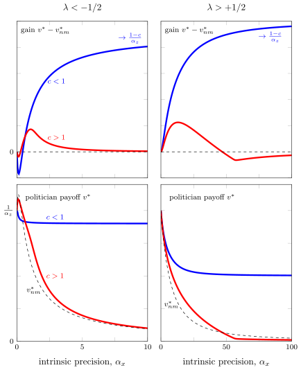
Politician’s benefit from manipulation \(v^*-v_{nm}^*\) (top row) and payoff \(v^*\) (bottom row) as functions of the intrinsic precision \(\alpha_x\) for various costs of manipulation \(c\) when the journalists’ actions are strong strategic substitutes \(\lambda<-1/2\) (left column) or strong strategic complements \(\lambda>1/2\) (right column). The politician’s payoff absent manipulation \(v_{nm}^*\) asymptotes to zero as \(\alpha_x\rightarrow\infty\). If \(c>1\) the politician’s payoff with manipulation \(v^*\) also asymptotes to zero but if \(c<1\) then \(v^*\) asymptotes to \((1-c)/\alpha_z>0\) so that the politician benefits. The politician benefits the most when when \(c\) is low and \(\alpha_x\) is high. In the left column we use \(\lambda<-1\) to highlight that for this parameter setting \(v^*\) and \(v_{nm}^*\) need not be monotonic in \(\alpha_x\).

Open this figure on its own page

A striking feature of Figure 8 is that the politician gains the most from manipulation when \(c\) is low and \(\alpha_x\) is high, regardless of \(\lambda\).

C.3 Journalists’ and Citizens’ Welfare

Journalists. We first define the journalists’ loss function \[\tag{C15} l_{\mathcal{J}}(\delta):=\min_{k\in[0,1]}\, L_{\mathcal{J}}(k,\delta)\] where \(L_{\mathcal{J}}(k,\delta)\) denotes the journalists’ ex-ante expected loss, i.e., the expectation of (40) in the main text with respect to the prior that \(\theta\) is normally distributed with mean \(z\) and precision \(\alpha_z\), if they choose \(k\) when the politician has manipulation \(\delta\). This works out to be \[\tag{C16} L_{\mathcal{J}}(k,\delta) = \frac{1-\lambda}{\alpha_z} B(\delta,k) + \frac{1}{\alpha_x}k^2\] where again \(B(\delta,k):=(k\delta+1-k)^2\) denotes the politician’s benefit from manipulation. Evaluating at the journalists’ best response \(k(\delta)\) and collecting terms gives \[\tag{C17} l_{\mathcal{J}}(\delta) = L_{\mathcal{J}}(k(\delta),\delta) = \frac{1}{\alpha_x}\,\left(\frac{k(\delta)}{1-\delta}\right) = \left(\frac{1}{1+\alpha(1-\delta)^2}\right)\frac{1-\lambda}{\alpha_z}.\]

Citizens. The citizens evaluate outcomes according to the loss \[\tag{C18} \int_0^1 (a_j-\theta)^2 \,dj = (A-\theta)^2 + \int_0^1 (a_j-A)^2 \,dj\] So the citizens are at their bliss point if the journalists all produce \(a_j=\theta\).

Now let \(L_{\mathcal{C}}(k,\delta)\) denote the citizens’ ex ante expected loss, i.e., the expectation of (C18) with respect to the prior that \(\theta\) is normally distributed with mean \(z\) and precision \(\alpha_z\), if the journalists choose \(k\) when the politician has manipulation \(\delta\). This works out to be \[\tag{C19} L_{\mathcal{C}}(k,\delta) = \frac{1}{\alpha_z}B(\delta,k) + \frac{1}{\alpha_x}k^2\] as in equation (30) in the main text.

Wedge between journalists’ and citizens’ losses. Comparing (C19) and (C16) we see that \[\tag{C20} L_{\mathcal{C}}(k,\delta) = L_{\mathcal{J}}(k,\delta) + \frac{\lambda}{\alpha_z} B(\delta,k)\] In the special case \(\lambda=0\), where the journalists care only about accurate reporting with no interactions amongst themselves, the citizens’ loss and the journalists’ loss coincide. More generally, since \(B(\delta,k)\geq0\), the citizens’ loss is larger than the journalists’ loss whenever \(\lambda>0\) and is less than the journalists’ loss whenever \(\lambda<0\). Intuitively, an incentive to coordinate, \(\lambda>0\), means that individual journalists respond more to their common prior \(z\) than its underlying precision warrants. Therefore, from the citizens’ point of view, the journalists are excessively responsive to their prior and hence under-responsive to the information contained in their signals. For example, if \(\lambda\rightarrow 1\) the journalists can be quite content when they are producing similar reports, \(a_i\approx A\), even if those reports are far from \(\theta\) and hence very unsatisfactory from the citizens’ point of view.

Effects of manipulation on journalists and citizens. Evaluating \(L_{\mathcal{J}}(k,\delta)\) at the journalists’ best response \(k(\delta)\) we can then write \[\tag{C21} l_{\mathcal{C}}(\delta):=L_{\mathcal{C}}(k(\delta),\delta) = l_{\mathcal{J}}(\delta) + \frac{\lambda \alpha_z}{(1-\lambda)^2} \, \,l_{\mathcal{J}}(\delta)^2\] The comparison of the citizens’ equilibrium loss with and without manipulation is then reduced to comparing \(l^*_{\mathcal{C}}=l_{\mathcal{C}}(\delta^*)\) and \(l^*_{\mathcal{C},nm}=l_{\mathcal{C}}(0)\). Similarly, the comparison of the journalists’ equilibrium loss with and without manipulation is reduced to comparing \(l^*_{\mathcal{J}}=l_{\mathcal{J}}(\delta^*)\) and \(l_{\mathcal{J},nm}^*=l_{\mathcal{J}}(0)\). Our main result here is:

So the journalists are always worse off with manipulation. Whether the citizens are worse off or not depends on the strategic interactions among the journalists. If the journalists’ actions are not strong strategic substitutes, \(\lambda>-1\), the citizens are also unambiguously worse off with manipulation. But if the journalists’ actions are strong strategic substitutes, \(\lambda<-1\), and if in addition the intrinsic precision of journalists’ signals is low enough, \(\alpha_x<\widehat{\alpha}^{\,**}_x\), then, perhaps surprisingly, the citizens are in fact better off with manipulation. To understand this, first notice that when \(\lambda<-1\), the journalists have a strong incentive to differentiate themselves from one another and their response \(k\) to their idiosyncratic signals is, from the citizens’ point of view, more than is warranted by the underlying precision of their signals. This is especially problematic for the citizens when the signals are imprecise, i.e., when \(\alpha_x\) is very low. By reducing \(k\), the politician’s manipulation then “corrects” for this, which makes the citizens better off than they would be absent manipulation.¹²

Effects of \(\alpha_x\) on journalists’ loss. Notice from the journalists’ loss function (C17) the strategic interaction term \((1-\lambda)\) and the prior precision \(\alpha_z\) simply scale the whole loss. Similar to the citizens’ loss (31) in the benchmark model, we can measure the equilibrium payoffs for the journalists, \(l^*_{\mathcal{J}}=l_{\mathcal{J}}(\delta^*)\), by their indirect utility evaluated at the equilibrium manipulation: \[\tag{C22} u^*(\alpha,c)=\alpha(1-\delta^*(\alpha,c))^2.\] This term is identical to (32) in the main text except that the composite precision parameter \(\alpha:=(1-\lambda)\alpha_x/\alpha_z\) now incorporates the effect of the strategic interactions. The welfare results on \(u^*(\alpha,c)\) in Proposition 3 and Remark 1 of the main text therefore also apply to the equilibrium payoffs of the journalists in the extended model. In the following corollary, we restate the welfare results in terms of the journalists’ loss and the intrinsic signal precision \(\alpha_x\):

Effects of \(\alpha_x\) on citizens’ loss. Evaluating the expression for the citizens’ loss in (C21) at the equilibrium manipulation \(\delta^*\) gives \[\tag{C23} l^*_{\mathcal{C}}= l^*_{\mathcal{J}} + \frac{\lambda\alpha_z}{(1-\lambda)^2} \, l_{\mathcal{J}}^{*\,2}\] Hence the effects of \(\alpha_x\) on the citizens’ equilibrium loss are given by the total derivative \[\tag{C24} \frac{d l^*_{\mathcal{C}}}{d\alpha_x} = \frac{d l^*_{\mathcal{J}}}{d\alpha_x} \bigg[1+\frac{2\lambda\alpha_z}{(1-\lambda)^2} \, l_{\mathcal{J}}^{*}\bigg]\] This expression is convenient because all the effects of \(\alpha_x\) enter \(l^*_{\mathcal{C}}\) only through \(l^*_{\mathcal{J}}\). This gives:

Figure 9 illustrates the effects of \(\alpha_x\) on the journalists’ and citizens’ loss. The left and right columns show the cases \(\lambda>-1\) and \(\lambda<-1\) respectively. The top and bottom rows show the cases \(c>1\) and \(c<1\) respectively. Each panel shows the loss of the citizens \(l^*_{\mathcal{C}}\) and the journalists \(l^*_{\mathcal{J}}\) as functions of \(\alpha_x\). The dashed lines demarcate the critical points \(\alpha_x^{**}\) and \(\underline{\alpha}_x^{**},\overline{\alpha}_x^{**}\). As with the journalists’ loss, the limit of the citizens’ loss as \(\alpha_x\rightarrow\infty\) is sensitive to the costs of manipulation \(c\). If \(c<1\), as \(\alpha_x\rightarrow\infty\) the citizens’s loss \(l^*_{\mathcal{C}}\) asymptotes to the same loss \(1/\alpha_z\) the citizens would have if \(\alpha_x=0\). If \(c>1\), the citizens’s loss \(l^*_{\mathcal{C}}\) asymptotes to zero, the same limit of the citizens’ loss without manipulation, \(l^*_{\mathcal{C},nm}\).

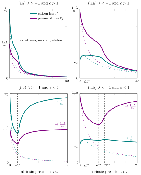
Citizens’ loss \(l_{\mathcal{C}}^*\) and journalists’ loss \(l_{\mathcal{J}}^*\) as functions of \(\alpha_x\) for \(c>1\) (top row) and \(c<1\) (bottom row) and for \(\lambda>-1\) (left column) and \(\lambda<-1\) (right column). If \(\lambda>-1\) both loss functions move in the same direction in response to \(\alpha_x\). If \(c>1\) both loss functions are strictly decreasing (top left). If \(c<1\) both loss functions are \(\cup\)-shaped with critical point \(\alpha_x^{**}\) (bottom left). If \(\lambda<-1\) the loss functions move in the same direction only between the critical points \(\underline{\alpha}_x^{**}\) and \(\overline{\alpha}_x^{**}\) (right column). If \(c<1\) the citizens’ loss asymptotes to \(1/\alpha_z\) and the journalists’ loss asymptotes to \((1-\lambda)/\alpha_z\). For the left column we use \(\lambda>0\) which implies that the journalists’ loss is less than the citizens’ loss. The colored dashed lines show the corresponding loss functions absent manipulation. If \(\lambda<-1\) then for \(\alpha_x\) sufficiently small the citizens are better off with manipulation.

Open this figure on its own page

D Heterogeneous Priors and Manipulation of the Signal Variance

In this appendix we provide further details on the extension where citizens have heterogeneous priors and where the politician can manipulate the signal variance.

Setup. Given that the citizens have linear strategies \(a(x_i,z_i)=kx_i + (1-k)z_i\) the politician’s problem is now to choose \(y\) and \(\gamma\) to maximize \[\begin{aligned} V(y,\gamma) & = \int_0^1 (k(y+\varepsilon_i) + (1-k)(z+\eta_i) - \theta)^2 \, di - c(y-\theta)^2 - c_{\gamma}(\gamma-1)^2 \\ & = (ky+(1-k)z - \theta)^2 + \gamma \sigma_x^2 k^2 + \sigma_{\eta}^2 (1-k)^2- c(y-\theta)^2 - c_{\gamma}(\gamma-1)^2 \end{aligned}\] The first order condition for the variance manipulation factor \(\gamma\) can be written \[\tag{D1} \gamma(k) = 1 + \frac{\sigma_x^2}{2c_{\gamma}}k^2\] And since the objective is separable in \(y\) and \(\gamma\) the first order condition for the signal mean \(y\) is as in the benchmark model \[\tag{D2} y(\theta) = (1-\delta)\theta + \delta z,\qquad \delta(k)=\frac{k-k^2}{c-k^2}\] where the second order condition again requires \(c-k^2\geq0\). The optimal action for the citizens is \(a_i=\mathbb{E}[\theta\,|\,x_i,z_i]\). The citizens have signals \(x_i=y+\varepsilon_i=(1-\delta)\theta+\delta z+\varepsilon_i\) and prior \(z_i=z+\eta_i=\theta+\varepsilon_{z}+\eta_i\). Using the properties of the bivariate normal distribution, conditional on \(x_i,z_i\) the citizens posterior for \(\theta\) is normal with expected value \[ \mathbb{E}[\theta\,|\,x_i,z_i] = \frac{(1-\delta)\sigma_z^2 + \sigma_{\eta}^2 }{(1-\delta)^2\sigma_z^2 + \sigma_{\eta}^2 + \gamma \sigma_x^2}\, x_i + \left(1- \frac{(1-\delta)\sigma_z^2 + \sigma_{\eta}^2 }{(1-\delta)^2\sigma_z^2 + \sigma_{\eta}^2 + \gamma \sigma_x^2}\right) \, z_i\] Hence indeed the citizens have strategies of the form \(a(x_i,z_i)=kx_i + (1-k)z_i\) where \[\tag{D3} k(\delta,\gamma) = \frac{(1-\delta)\sigma_z^2 + \sigma_{\eta}^2 }{(1-\delta)^2\sigma_z^2 + \sigma_{\eta}^2 + \gamma \sigma_x^2}\]

Equilibrium.

Comparative statics.

“Regime changes" in the amount of manipulation. First we define the mapping: \[\tag{D14} F\left( k,\sigma _{z}^{2},\sigma _{x}^{2},\sigma _{\eta}^{2},c_{\gamma}\right) :=\frac{\sigma _{z}^{2}}{\sigma _{z}^{2}+\sigma _{x}^{4} \, k^{3}\left( 1+k\right) /c_{\gamma}+\sigma _{\eta}^{2}\left( 1+k\right) }\] To facilitate some comparisons, in some of the expressions below we return to precision notation \(\alpha_x=1/\sigma_x^2\) and \(\alpha_z=1/\sigma_z^2\) with relative precision \(\alpha=\alpha_x/\alpha_z\) etc. With this notation in mind we then have a result analogous to Proposition 2 in the main text:

E Weights on Components of Citizens’ Loss Function

In this appendix, we discuss a further extension to our benchmark model that allows the citizens to have different weights on the \((a_i-\theta)^2\) and \((A-\theta)^2\) terms in their loss function (in other words, allows the citizens to weigh these discord and disinformation terms differently to the policitican). In particular, suppose each citizen seeks to minimize the expected loss \[\tag{E1} l_{i}=(a_{i}-\theta )^{2}+\omega (A-\theta )^{2}\]The weight \(\omega\) does not affect their optimal action so we still have the usual \[\tag{E2} a_i=kx_{i}+(1-k)z\]where \(k\) is given by \[\tag{E3} k(\delta )=\frac{(1-\delta)\alpha}{(1-\delta)^{2}\alpha +1},\qquad \alpha :=\alpha _{x}/\alpha _{z}\] The weight \(\omega\) plays no role in determining the equilibrium outcomes \(k^*,\delta^*\) but it does affect how those outcomes are evaluated. The citizens’ ex ante expected loss is now \[\tag{E4} L(k,\delta;\omega) =\frac{1+\omega }{\alpha _{z}}B(k,\delta )+\frac{1}{\alpha _{x}}k^{2}\]where as usual \(B(k,\delta )=(k\delta +1-k)^{2}\). Notice that \(\omega =0\) is our benchmark model. Now write this as \[\tag{E5} L(k,\delta;\omega)=L(k,\delta;0)+\frac{\omega }{\alpha _{z}}B(k,\delta ).\]And recall that at the best response \[\tag{E6} B(k(\delta ),\delta )=(1-k(\delta )\left( 1-\delta \right) )^{2}=\left( \frac{k(\delta )}{\alpha (1-\delta )}\right) ^{2}\]so that we can write\[\tag{E7} L(k,\delta;0)=\frac{1}{\alpha _{x}}\frac{k(\delta )}{1-\delta }.\]which then implies \[\tag{E8} B(k(\delta ),\delta )=\left( \frac{\alpha _{x}}{\alpha }L(k,\delta;0)\right) ^{2}=\left( \alpha _{z}L(k,\delta;0)\right) ^{2}\]so that we can then write \[L(k,\delta;\omega )=L(k,\delta;0)+\omega \alpha _{z}L(k,\delta;0)^{2} \tag{E9}\] Now let \(l^*(\omega):=L(k^*,\delta^*;\omega)\). In this notation \(l^*(0)\) is the citizens’ loss in our benchmark model. We then have the following welfare result analogous to Supplementary Proposition 4 in Appendix C above.

F Omitted Proofs

In this appendix we provide proofs of results hitherto omitted. We first state and prove two supplementary lemmas used in proof of Proposition 3 in the main text. We then provide proofs of the supplemantary propositions in the extension with active media in Appendix C above.

F.1 Further Details from Proof of Proposition 3 in Main Text

F.2 Proofs of Additional Results from Extension with Active Media

Proof of Supplementary Proposition 1

Using the fixed point condition (A2) with the redefined \(\alpha = (1-\lambda)\alpha_{x}/\alpha_{z}\), we can write \[\tag{F21} v^*=\frac{1}{(1-\lambda)\alpha_x} \left\{ k^*-\lambda k^{*2} + \frac{k^{*2}(1-k^*)^2}{c-k^*} \right\}\] Using the analogous condition for \(k_{nm}^*\), we can write \[\tag{F22} v^*_{nm} = \frac{1}{(1-\lambda)\alpha_x} \left\{ k_{nm}^*-\lambda k_{nm}^{*2} \right\}\] Hence the politician’s manipulation backfires, \(v^*<v_{nm}^*\), if and only if \[\tag{F23} g(k^*) < f(k_{nm}^*) - f(k^*)\] where \[\tag{F24} f(k):=k-\lambda k^2,\qquad g(k):=\frac{k^2(1-k)^2}{c-k}\geq0\]

For part (i) suppose that \(\lambda<0\). We know from (C8) and (C9) that a necessary condition for the politician’s manipulation to backfire is \(k<k^*_{nm}\). We can rewrite the inequality in (F23) as \[\tag{F25} \frac{k^{*2}(1-k^*)^2}{c-k^*}<(k^*_{nm}-k)(1-\lambda(k^*_{nm}+k^*))\] Using the fixed point conditions (A2) for both \(k^*\) and \(k_{nm}^*\), we can rewrite the key condition (F25) as \[\tag{F26} \lambda< \frac{1}{c-k^*}\,\frac{K_1 K_2 }{K_3 K_4}\] where \[\begin{aligned} K_1 &:= 4ck^{*2} - c^2 - k^{*3} - 2ck^{*3} - k^{*4} + k^{*5} \\ K_2 &:= c(c-k^*)(1-k^*)+k^*(c-k^{*2})^2 > 0 \\ K_3 &:= k^{*3}-2ck^*+c > 0 \\ K_4 &:= (1+k^*)(c-k^{*2})^2 + c(c-k^*)(1-k^*) > 0 \end{aligned}\] Now consider taking \(\alpha_x\rightarrow 0\) for fixed \(\lambda<0\) such that \(k^*\rightarrow 0\). We then have the following limits \[ K_1 \rightarrow -c^2,\quad K_2 \rightarrow +c^2,\quad K_3 \rightarrow c, \quad K_4 \rightarrow 2c^2\] So in the limit the RHS of (F26) is \[\tag{F27} \frac{1}{c-k^*}\,\frac{K_1 K_2 }{K_3 K_4} \rightarrow \frac{1}{(c-0)}\,\frac{(-c^2)(c^2)}{(c)(2c^2)} = -\frac{1}{2}\] Hence for any \(\lambda<-1/2\) we can find \(\alpha_x\) sufficiently close to zero such that (F26) is satisfied and in turn the politician’s manipulation backfires, \(v^*<v^*_{nm}\).

For part (ii), suppose that \(\lambda>0\). We know from (C8) and (C9) that the necessary condition for the politician’s manipulation to backfire is \(k^*>k_{nm}^*\). We can rewrite the inequality in (F23) as \[\tag{F28} \frac{k^{*2}(1-k^*)^2}{k^*-k_{nm}^*} < (\lambda (k_{nm}^*+k^*)-1))(c-k^*)\] Using the fixed point conditions (A2) for both \(k^*\) and \(k_{nm}^*\), we can rewrite this key condition as \[\tag{F29} \frac{k^{*2}(1-k^*)}{\frac{k_{nm}^*}{k^*}\left(c\frac{(c-k^*)}{(c-k^{*2})^2}\right)-1} < (\lambda (k_{nm}^*+k^*)-1))(c-k^*)\] Observe that if, in addition, \(c>1\) and \(\lambda>1/2\), then the RHS of (F29) converges to a strictly positive constant \[\tag{F30} \lim_{\alpha_x\rightarrow\infty} (\lambda (k_{nm}^*+k^*)-1))(c-k^*) = (\lambda 2-1)(c-1)>0\] (since \(k^*\rightarrow 1\) if \(c>1\)). But the LHS of (F29) converges to zero \[\tag{F31} \lim_{\alpha_x\rightarrow\infty} \frac{k^{*2}(1-k^*)}{\frac{k_{nm}^*}{k^*}c\frac{c-k^*}{(c-k^{*2})^2}-1} = \frac{0^+}{\frac{c}{(c-1)}-1} = 0^+\] Therefore, if \(k^*>k_{nm}^*\), \(c>1\) and \(\lambda>1/2\) then there exists \(\alpha_x^*\) such that for \(\alpha_x>\alpha_x^*\) the LHS of (F29) is strictly less than the RHS of (F29) so that the politician’s manipulation backfires, \(v^*<v_{nm}^*\).

Finally, we know from Remark 2 that \(k^*<k_{nm}^*\) if and only if \(c<c^*_{nm}(\alpha)\). Also observe that \(c<1\) is sufficient for \(c<c^*_{nm}(\alpha)\) if \(1<c^*_{nm}(\alpha)\). From (C11) we have \(1<c^*_{nm}(\alpha)\) if \(\alpha<1\), or if \(\alpha>1\) and \(\alpha<(1+\sqrt{5})/2\). Since \(\alpha=(1-\lambda)\alpha_x/\alpha_z\), the critical point \(\underline{\alpha}_x^*\) must be \[\tag{F32} \underline{\alpha}_x^*<\bigg(\frac{1+\sqrt{5}}{2}\bigg)\bigg(\frac{\alpha_z}{1-\lambda}\bigg)\] Likewise, \(c>1\) is sufficient condition for \(c>c^*_{nm}(\alpha)\) if \(1>c^*_{nm}(\alpha)\), and we need \(\alpha>(1+\sqrt{5})/2\) to ensure that \(1>c^*_{nm}(\alpha)\). Since \(\alpha=(1-\lambda)\alpha_x/\alpha_z\), the critical point \(\overline{\alpha}_x^*\) must be \[\tag{F33} \overline{\alpha}_x^*>\bigg(\frac{1+\sqrt{5}}{2}\bigg)\bigg(\frac{\alpha_z}{1-\lambda}\bigg)\]

\(\hfill \square\)

Proof of Supplementary Proposition 3.

For part(i), \(l_{\mathcal{J}}(\delta)\) is increasing in \(\delta\) from equation (C17). Hence, \(l_{\mathcal{J}}(\delta^*) > l_{\mathcal{J}}(0)\) whenever \(\delta^*>0\). We then have that the journalists are unambiguously worse off when the politician can manipulate. For part (ii) use \(l^*_{\mathcal{C}}=l_{\mathcal{C}}(\delta^*)\) and equation (C21) to write \[\tag{F34} l_{\mathcal{C}}^* = l_{\mathcal{J}}(\delta^*) + \frac{\lambda \alpha_z}{(1-\lambda)^2} \, \,l_{\mathcal{J}}(\delta^*)^2\] and likewise \[\tag{F35} l_{\mathcal{C},nm}^* = l_{\mathcal{J}}(0) + \frac{\lambda \alpha_z}{(1-\lambda)^2} \, \,l_{\mathcal{J}}(0)^2\] Differencing these expressions we can write \[\tag{F36} l_{\mathcal{C}}^* - l_{\mathcal{C},nm}^* = \Big(l_{\mathcal{J}}(\delta^*) - l_{\mathcal{J}}(0) \Big)\times\left[1+\frac{\lambda \alpha_z}{(1-\lambda)^2}\Big(l_{\mathcal{J}}(\delta^*) + l_{\mathcal{J}}(0) \Big) \right]\] Now write the term in square brackets on the LHS as \(\Delta(\delta^*)\) where \(\Delta(\delta)\) is the function \[\tag{F37} \Delta(\delta):=1+\frac{\lambda \alpha_z}{(1-\lambda)^2}\Big(l_{\mathcal{J}}(\delta) + l_{\mathcal{J}}(0) \Big)\] From part (i) we know \(l_{\mathcal{J}}(\delta^*) > l_{\mathcal{J}}(0)\) so \(l_{\mathcal{C}}^* > l_{\mathcal{C},nm}^*\) if and only if \(\Delta(\delta^*)>0\). Since \(\alpha_z>0\) and \(l_{\mathcal{J}}(\delta^*)>l_{\mathcal{J}}(0)>0\), a sufficient condition for \(\Delta(\delta^*)>0\) is that \(\lambda>0\). To prove part (ii) we need to show that any \(\lambda>-1\) is also sufficient. To see this, observe that since \(l_{\mathcal{J}}(\delta)\) is strictly increasing in \(\delta\), for \(\lambda<0\) we also know that \(\Delta(\delta)\) is strictly decreasing in \(\delta\) which in turn implies \(\Delta(\delta)\geq \Delta(1)\). Hence if \(\lambda<0\) a sufficient condition for \(\Delta(\delta^*)>0\) is that \(\Delta(1)>0\). Calculating \(\Delta(1)\) gives \[\begin{aligned} \Delta(1) & = 1+\frac{\lambda \alpha_z}{(1-\lambda)^2}\Big(l_{\mathcal{J}}(1) + l_{\mathcal{J}}(0) \Big) \\ & = 1+\frac{\lambda \alpha_z}{(1-\lambda)^2}\Big(\frac{1-\lambda}{\alpha_z} + \frac{1-\lambda}{(1-\lambda)\alpha_x+\alpha_z} \Big) \end{aligned}\] where the second equality follows from the expression for \(l_{\mathcal{J}}(\delta)\) in equation (C17) evaluated at \(\delta=1\) and \(\delta=0\). Simplifying further \[\tag{F38} \Delta(1) = 1+\frac{\lambda}{1-\lambda}\Big(1 + \frac{1}{1+\alpha} \Big)\] where \(\alpha:=(1-\lambda)\alpha_x/\alpha_z>0\). So for \(\lambda<0\) a sufficient condition for \(\Delta(1)>0\) and hence \(\Delta(\delta^*)>0\) is \[\tag{F39} \frac{\lambda}{1-\lambda}\Big(1 + \frac{1}{1+\alpha} \Big) > - 1\] or equivalently \[\tag{F40} 1+\alpha > - \lambda\] Since \(\alpha>0\) a sufficient condition for this is \(\lambda>-1\). To summarize, any \(\lambda>-1\) is sufficient for \(\Delta(\delta^*)>0\) and hence sufficient for \(l_{\mathcal{C}}^* > l_{\mathcal{C},nm}^*\). For part (iii) we then know that \(\lambda<-1\) is necessary for \(l_{\mathcal{C}}^* < l_{\mathcal{C},nm}^*\). Recall that \(\Delta(\delta)\) is strictly decreasing in \(\delta\), i.e., \(\Delta(\delta)\leq \Delta(0)\), for \(\lambda<0\). Hence for \(\lambda<-1\) a sufficient condition for \(\Delta(\delta^*)<0\) is that \(\Delta(0)<0\). Calculating \(\Delta(0)\) gives \[\begin{aligned} \Delta(0) & = 1+\frac{\lambda \alpha_z}{(1-\lambda)^2}\Big(l_{\mathcal{J}}(0) + l_{\mathcal{J}}(0) \Big) \\ & = 1+\frac{\lambda \alpha_z}{(1-\lambda)^2}\Big(\frac{2(1-\lambda)}{(1-\lambda)\alpha_x+\alpha_z} \Big) \\ & = 1+\frac{\lambda}{1-\lambda}\Big(\frac{2}{1+\alpha} \Big) \end{aligned}\] So for \(\lambda<-1\) a sufficient condition for \(\Delta(0)<0\) and hence \(\Delta(\delta^*)<0\) is \[\tag{F41} \alpha < \frac{\lambda+1}{\lambda-1} = - \left(\frac{1+\lambda}{1-\lambda}\right), \qquad \lambda<-1\] Since \(\alpha:=(1-\lambda)\alpha_x/\alpha_z>0\) we rewrite this as \[\tag{F42} \alpha_x < \widehat{\alpha}_{x}^{**} := - \left(\frac{1+\lambda}{(1-\lambda)^2} \right)\, \alpha_z,\qquad \lambda<-1\] To summarize, for each \(\lambda<-1\) there is a critical point \(\widehat{\alpha}_{x}^{**}\) such that together \(\lambda<-1\) and \(\alpha_x<\widehat{\alpha}_{x}^{**}\) are sufficient for \(\Delta(\delta^*)<\Delta(0)<0\) and hence sufficient for \(l_{\mathcal{C}}^* < l_{\mathcal{C},nm}^*\). \(\hfill \square\)

Proof of Supplementary Proposition 4.

From equation (C24) we see that the derivative of \(l_{\mathcal{C}}^{*}\) with respect to \(\alpha_x\) and the derivative of \(l_{\mathcal{J}}^{*}\) with respect to \(\alpha_x\) have the same sign if and only if \[\tag{F43} 1+\frac{2\lambda\alpha_z}{(1-\lambda)^2} \, l_{\mathcal{J}}^{*} > 0\] Write this key term \(T(\delta^*)>0\) where \[\tag{F44} T(\delta) := 1+\frac{2\lambda\alpha_z}{(1-\lambda)^2} \, l_{\mathcal{J}}(\delta)\] Clearly \(\lambda \geq 0\) suffices for \(T(\delta^*)>0\). When \(\lambda<0\), \(T(\delta^*)>0\) if and only if \[\tag{F45} l_{\mathcal{J}}^* < -\frac{(1-\lambda)^2}{2\lambda\alpha_z}:=l_{crit}\] From Proposition 3 and Remark 1 we know that the maximum of \(l_{\mathcal{J}}^*\) is \(l^*_{max}={(1-\lambda)}/{\alpha_z}\). If \(l^*_{max}<l_{crit}\), i.e., if \(\lambda\in(-1,0)\), the inequality (F45) holds and therefore \(T(\delta^*)>0\). Alternatively, if \(l^*_{max}>l_{crit}\), i.e., if \(\lambda\in(-\infty,-1)\), there exists a subset of \(\alpha_x\) such that the inequality (F45) does not hold and in turn \(T(\delta^*)<0\).

We now determine the set of \(\alpha_x\) such that (F45) does not hold, conditional on \(\lambda<-1\). For any \(c>1\) we know from Proposition 3 and Remark 1 that \(l_{\mathcal{J}}^*\) is strictly decreasing in \(\alpha_x\) with \(\lim_{\alpha_x\rightarrow 0^+} l^*_{\mathcal{J}}=l^*_{max}\) and \(\lim_{\alpha_x\rightarrow \infty} l^*_{\mathcal{J}} =0\). Hence for each \(\lambda<-1\) and \(c>1\) there is a unique critical point \(\underline{\alpha}_x^{**}>0\) such that \(T(\delta^*)>0\) if and only if \(\alpha_x>\underline{\alpha}_x^{**}\). Similarly, for any \(c<1\) we again know from Proposition 3 and Remark 1 that \(l_{\mathcal{J}}^*\) is strictly decreasing in \(\alpha_x\) if and only if \(\alpha_x<\alpha_x^{**}\) and \(\lim_{\alpha_x\rightarrow 0^+} l^*_{\mathcal{J}}=\lim_{\alpha_x\rightarrow \infty} l^*_{\mathcal{J}} =l^*_{max}\). Let \(l_{min}^*\) denote the journalists’ loss at the \(\alpha_x=\alpha_x^{**}\) that achieves the minimum. For any \(c<1\) and any fixed loss \(l\in(l_{min}^*,l_{max}^*)\) there are two critical points \(\underline{\alpha}_x(l)<\alpha_x^{**}<\overline{\alpha}_x(l)\) such that \(l_{\mathcal{J}}^*<l\) if and only if \(\alpha_x\in(\underline{\alpha}_x(l),\overline{\alpha}_x(l))\). Then for each \(\lambda<-1\) and \(c<1\) there are two possibilities, either \(l_{crit}\in(l_{min}^*,l_{max}^*)\) or \(l_{crit}\leq l_{min}^*\). For the interior cases \(l_{crit}\in(l_{min}^*,l_{max}^*)\) we define the critical points by \(\underline{\alpha}_x^{**}:=\underline{\alpha}_x(l_{crit})\) and \(\overline{\alpha}_x^{**}:=\overline{\alpha}_x(l_{crit})\). For the boundary case \(l_{crit}\leq l_{min}^*\) we define the critical points by \(\underline{\alpha}_x^{**}=\overline{\alpha}_x^{**}=+\infty\). Given these critical points, we have \(T(\delta^*)>0\) if and only if \(\alpha_x \in(\underline{\alpha}_x^{**},\overline{\alpha}_x^{**})\). \(\hfill \square\)

G Knife-Edge Case \(c=1\)

In this appendix we discuss the technicalities that arise when the costs of manipulation \(c=1\) exactly.

Preliminaries. There is no issue with \(c=1\) if the relative precision \(\alpha\leq 4\). The issues with \(c=1\) arise only if \(\alpha>4\). To see this, first recall from Lemma 1 that if \(\alpha>1\) the citizens’ best response \(k(\delta;\alpha)\) is increasing in \(\delta\) on the interval \([0,\hat{\delta}(\alpha)]\) and obtains its maximum at \(\delta=\hat{\delta}(\alpha)=1-1/\sqrt{\alpha}\in(0,1)\). At the maximum, the citizens’ best response takes on the value \(k(\hat{\delta}(\alpha);\alpha)=\sqrt{\alpha}/2\). Hence for \(\alpha>4\) the maximum value exceeds \(1\). Moreover, by continuity of the best response in \(\delta\) if \(\alpha>4\) there is an interval of \(\delta\) such that \(k(\delta;\alpha)>1\). The boundaries of this interval \((\underline{\delta}(\alpha),\overline{\delta}(\alpha))\) are given by the roots of \(k(\delta;\alpha)=1\), which work out to be \[\tag{G1} \underline{\delta}(\alpha) \, , \, \overline{\delta}(\alpha) = \frac{1}{2}\bigg(1 \pm \sqrt{1-(4/\alpha)}\bigg),\qquad \alpha\geq 4\] Observe that this interval is symmetric and centred on \(1/2\) with a width of \[\tag{G2} \overline{\delta}(\alpha)-\underline{\delta}(\alpha) = \sqrt{1-(4/\alpha)}\geq0,\qquad \alpha\geq 4\] If \(\alpha=4\), we have \(\underline{\delta}(4)=\overline{\delta}(4)=1/2\) but as \(\alpha\) increases the width of the interval \((\underline{\delta}(\alpha),\overline{\delta}(\alpha))\) expands around \(1/2\) with the boundaries \(\underline{\delta}(\alpha)\rightarrow 0^{+}\) and \(\overline{\delta}(\alpha)\rightarrow 1^-\) as \(\alpha\rightarrow\infty\). Now recall from Proposition 1 that only \(k\in[0,\min(c,1)]\) and \(\delta\in[0,1]\) are candidates for an equilibrium. So if \(\alpha>4\) then none of the values of \(\delta\in(\underline{\delta}(\alpha),\overline{\delta}(\alpha))\) are candidates for an equilibrium.

Costs of manipulation, \(c \neq 1\). Now consider the politician’s best response \(\delta(k;c)\) parameterized by \(c \neq 1\) and suppose \(\alpha>4\). When \(c \neq 1\), the politician’s objective depends on \(\delta\) over the entire support \(k \in[0,\min(c,1)]\). From Proposition 1, there is a unique intersection between the politician’s and the citizens’ best responses. As illustrated below, if \(c<1\) the politician’s best response \(\delta(k;c<1)\) lies above \(\delta(k;1)=k/(1+k)\) and hence the equilibrium point \(k^*,\delta^*\) must be on the “upper branch” of \(k(\delta;\alpha)\) where \(\delta^*>\overline{\delta}(\alpha)\). But for the same value of \(\alpha\) and instead \(c>1\) the equilibrium point \(k^*,\delta^*\) must be on the “lower branch” of \(k(\delta;\alpha)\) where \(\delta^*<\underline{\delta}(\alpha)\) because the politician’s best response \(\delta(k;c>1)\) lies below \(\delta(k;1)=k/(1+k)\).

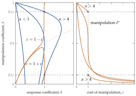
The left panel shows the citizens’ best response \(k(\delta;\alpha)\) for \(\alpha<1\), \(\alpha=4\) and \(\alpha>4\) (blue) and the politician’s best response \(\delta(k;c)\) for \(c=1-\varepsilon\), \(c=1\), and \(c=1+\varepsilon\) (red). For \(\alpha>4\), in the limit as \(c\rightarrow 1^-\) the equilibrium is at \(k^*=1,\delta^*=\overline{\delta}(\alpha)\) but in the limit as \(c\rightarrow 1^+\) the equilibrium is at \(k^*=1,\delta^*=\underline{\delta}(\alpha)\). For \(\alpha>4\) and \(c=1\) exactly both of these are equilibria because for this knife-edge special case the politician is indifferent between \(\underline{\delta}(\alpha)\) and \(\overline{\delta}(\alpha)\). The right panel shows the equilibrium manipulation \(\delta^*\) as a function of \(c\) for \(\alpha<1\), \(\alpha=4\) and \(\alpha>4\). For \(\alpha\leq 4\), the manipulation \(\delta^*\) is continuous in \(c\). But for \(\alpha>4\) the manipulation jumps discontinuously at \(c=1\). In the limit as \(\alpha\rightarrow\infty\) the boundaries \(\underline{\delta}(\alpha)\rightarrow 0^+\) and \(\overline{\delta}(\alpha)\rightarrow 1^+\) so that the manipulation jumps by the maximum possible amount, from \(\delta^*=0\) if \(c<1\) to \(\delta^*=1\) if \(c>1\).

Open this figure on its own page

Summary. In brief, when \(\alpha>4\) for each \(c<1\) the equilibrium \(\delta^*>\overline{\delta}(\alpha)\) with \(\delta^*\rightarrow \overline{\delta}(\alpha)\) from above as \(c\rightarrow 1^{-}\) and for each \(c>1\) the equilibrium \(\delta^*<\underline{\delta}(\alpha)\) with \(\delta^*\rightarrow \overline{\delta}(\alpha)\) from below as \(c\rightarrow 1^{+}\).

Knife-edge case. Now consider the case \(c=1\) exactly. The key part of the politician’s objective becomes \[\tag{G3} B(\delta,k)-C(\delta) = (k^2-1)\delta^2 + 2k(1-k)\delta + (1-k)^2\] When \(k \neq 1\), the politician’s best response is \(\delta(k;1)=k/(1+k)\), which is increasing in \(k\) and approaches 1/2 as \(k \rightarrow 1\). But when \(k=1\), the politician’s objective is independent of \(\delta\) and in turn the politician is indifferent in the choice of \(\delta\). The equilibrium \((k^*=1,\delta^*)\) is thus entirely determined by the citizens’ best response. If \(\alpha<4\), the citizens’ best response \(k(\delta;\alpha)<1\) so that \(k^*=1\) is never an equilibrium. If \(\alpha=4\), there is a unique equilibrium determined by the maximum of the citizens’ best response \((k^*=1,\delta^*=1/2)\). If \(\alpha>4\), there are two equilibria corresponding to the two roots of \(k(\delta;\alpha)=1\): namely \((k^*=1,\delta^*=\underline{\delta}(\alpha))\) and \((k^*=1,\delta^*=\overline{\delta}(\alpha))\).

Further intuition for large changes in manipulation near \(c=1\). Now consider the sensitivity of the equilibrium amount of manipulation to changes in \(c\) near \(c=1\). Recall that, taking the citizens’ \(k\) as given, the politician chooses manipulation \(\delta\) to maximize \[\tag{G4} V(\delta,k) = \frac{1}{\alpha_z} \, (B(\delta,k)-C(\delta)) + \frac{1}{\alpha_x}k^2\] with benefit \(B(\delta,k)=(k\delta+1-k)^2\) and costs of manipulation \(C(\delta)=c\delta^2\).

Now consider an environment where the citizens are inclined to be very responsive to their signals, \(\alpha\rightarrow\infty\) so that \(k\rightarrow \min(c,1)\). First, suppose that \(c>1\) so that \(k\rightarrow 1\). Then the relevant part of the politician’s objective simplifies to \[\tag{G5} B(\delta,1)-C(\delta) = (1-c)\delta^2\] so that for any \(c>1\) the politician will choose \(\delta=0\). Next, suppose instead that \(c<1\) so that \(k\rightarrow c\). In this case the relevant part of the politician’s objective simplifies to \[\tag{G6} B(\delta,c)-C(\delta) = -c(1-c)\delta^2 +2c(1-c)\delta + (1-c)^2\] so that for any \(c<1\) the politician will choose \(\delta=1\). In short, as \(\alpha\rightarrow\infty\), the politician’s manipulation is a step function in \(c\), with \(\delta=1\) for all \(c<1\) and \(\delta=0\) for all \(c>1\).

What is the meaning of \(c=1\)? So given that the amount of manipulation can be extremely sensitive to \(c\) near \(c=1\), what does \(c=1\) mean? Recall that in the politician’s objective (5) the gross benefit \(\int_0^1 (a_i-\theta)^2\, di\) has a coefficient normalized to \(1\). If instead we had written the objective with \(b\int_0^1 (a_i-\theta)^2\, di\) for some \(b>0\) then throughout the analysis the relevant parameter would be the cost/benefit ratio \(c/b\) and the critical point would be where the cost/benefit ratio is \(c/b=1\). In this parameterization, the politician’s equilibrium manipulation is extremely sensitive to changes in either \(c\) or \(b\) in the vicinity of \(c/b=1\). With \(\alpha\) high and costs and benefits evenly poised, a small decrease in \(b\) or small increase in \(c\) would lead to a large reduction in manipulation.

H Coefficients Sum to One

In this appendix we show that writing the citizens’ linear strategy as \(a_i=kx_i+(1-k)z\) is without loss of generality. Suppose that the citizens’ linear strategy is \[ a_i = \beta_0 + \beta_1 x_i + \beta_2 z\] for some coefficients \(\beta_0,\beta_1,\beta_2\). We will show that in any linear equilibrium \(\beta_0=0\) and \(\beta_1+\beta_2=1\).

The politician’s problem is then to choose \(y\) to maximize \[\begin{aligned} V(y) &= \int_0^1 \left(\beta_0 + \beta_1 (y+\varepsilon_i)+ \beta_2 z-\theta\right)^2 \, di - c(y-\theta)^2 \\ &= (\beta_0 + \beta_1 y + \beta_2 z-\theta)^2 + \frac{1}{\alpha_x}\beta_1^2 - c(y-\theta)^2 \end{aligned}\] The solution to this problem is \[ y = \gamma_0 + \gamma_1 \theta + \gamma_2 z\] where \begin{align} \gamma_0 = \frac{\beta_0\beta_1}{c-\beta_1^2} \tag{H1} \\ \gamma_1 = \frac{c-\beta_1}{c-\beta_1^2} \tag{H2} \\ \gamma_2 = \frac{\beta_1\beta_2}{c-\beta_1^2} \tag{H3} \end{align}

But if the politician has the strategy \(y = \gamma_0 + \gamma_1 \theta + \gamma_2 z\), the citizens’ posterior expectation of \(\theta\), and hence their action \(a_i\), is given by \[\begin{aligned} a_i=\mathbb{E}[\theta\,|\,x_i] &= \frac{\gamma_1 \alpha_x}{\gamma_1^2\alpha_x+\alpha_z}\left(\frac{1}{\gamma_1}(x_i-\gamma_2 z)-\frac{\gamma_0}{\gamma_1} \right) + \frac{\alpha_z}{\gamma_1^2\alpha_x+\alpha_z} z\\ &=\frac{\gamma_1\alpha_x}{\gamma_1^2\alpha_x+\alpha_z}x_i + \frac{\alpha_z-\gamma_1\alpha_x\gamma_2}{\gamma_1^2\alpha_x+\alpha_z}z-\frac{\gamma_1\alpha_x}{\gamma_1^2\alpha_x+\alpha_z}\gamma_0 \end{aligned}\] Matching coefficients with \(a_i=\beta_0+\beta_1 x_i + \beta_2 z\) we then have \begin{align} \beta_0 &= - \frac{\gamma_1\alpha_x}{\gamma_1^2\alpha_x+\alpha_z}\gamma_0 \tag{H4}\\ \beta_1 &= \phantom{-} \frac{\gamma_1\alpha_x}{\gamma_1^2\alpha_x+\alpha_z} \tag{H5}\\ \beta_2 &= \phantom{-} \frac{\alpha_z-\gamma_1\alpha_x\gamma_2}{\gamma_1^2\alpha_x+\alpha_z}\tag{H6} \end{align} First observe that equations (H1) and (H4) together imply that the intercepts are \(\beta_0=\gamma_0=0\). Then observe from (H2)-(H3) and (H5)-(H6) that \(\gamma_1+\gamma_2=1\) implies \(\beta_1+\beta_2=1\) and vice-versa. So indeed the citizens’ strategy takes the form \(a_i=kx_i + (1-k)z\) where \(k=\beta_1\) and the politician’s strategy takes the form \(y=(1-\delta)\theta+\delta z\) where \(\delta=\gamma_2\). Hence from (H3) and (H5) we can write \[ \delta = \frac{k-k^2}{c-k^2},\qquad \qquad k = \frac{(1-\delta)\alpha}{(1-\delta)^2\alpha+1}\] where \(\alpha:=\alpha_x/\alpha_z\). These are the same as the best response formulas equations (13) and (18) in the main text and from Proposition 1 we know that there is a unique pair \(k^*,\delta^*\) satisfying these conditions.