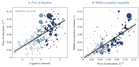
Each point is a three-digit occupation \(j\). Panel A plots the within-occupation price of education \(\beta_{j}^{\rm edu}\) against the occupation’s Autor and Dorn (2013) measure of cognitive task intensity. The weighted fit has gradient \(+0.015\). Panel B plots within-occupation variance \(V_j\) against the price of education \(\beta_{j}^{\rm edu}\). The weighted fit has gradient \(+0.710\). The within-occupation variance \(V_j = \boldsymbol{\beta}_j'\boldsymbol{\Sigma}_j\boldsymbol{\beta}_j\) where \(\boldsymbol{\Sigma}_{j}\) is the covariance matrix of the observed skills \(\boldsymbol{x}_{i}=(\mathrm{edu}_{i},\,\exp_{i},\,\exp_{i}^2)\) among workers in occupation \(j\). The Mincer regression (48) also controls for sex, race, and log hours with occupation-specific coefficients. Marker area is proportional to occupation sample size and marker color indicates terciles of cognitive task intensity. The shaded regions are pointwise \(95\%\) confidence bands. For visual clarity the panels are clipped to the employment-weighted 1st–99th percentile of the plotted variables. The four observations outside the frame in Panel A are those with negative estimated education prices, accounting for 0.2% of employment; a further 1.2% of employment lies outside the frame in Panel B. All of these outliers are retained in all estimation. ACS 2010 cross-section, \(J = 287\) occupations.